FW 453 Exam 2

Detectability: C = pN

N = abundance, C = Count Statistic, p = detection probability

Lincoln-Petersen Method

-Capture, mark, and release a sample of individuals from a population, then go back and recapture at a later date

-Proportion of marked individuals at second sample indicates the portion of the total population

Batch Marking

Groups of animals given the same mark

Lincoln-Petersen estimator: N= (n1n2)/m2

Estimates abundance, N = Abundance, n1 = individuals marked at occasion 1, n2 = individuals caught at occasion 2, m2 = marked individuals caught at occasion 2

Lincoln-Petersen estimator adjusted for bias

At smaller sample sites when the number of recaptures could be zero, N= [(n1+1)(n2+2)/(m2+1)]-1

Overall Detection Probability

p = m2/n2, probability = marked individuals caught at occasion 2/individuals captured at occasion 2

Lincoln-Petersen Assumptions

-closed population

-all animals have the same probability of being caught

-there is no tag loss or other loss of marks

Closed Populations

-Abundance is constant

-No gains or losses

-Most models

Open Populations

-Abundance may be constant or change

-Subject to gains and losses

-Estimate survival, recruitment, movement, etc... if sampling is well designed

Assumption of equal detection

-All animals have the same probability of being caught within an occasion

-Impacts could be: sampling technique, gear, time of year, home range differences between sexes

Violations of equal detection

Trap happy: more likely, probability increases, N decreases

Trap shy: less likely, probability decreases, N increases

Individual Marking

-Extra information

-Relax L-P assumptions

-More complex models and account for variation

Multiple Sample Capture-Mark-Recapture

-2 or more occasions

-More data to estimate, more precision

-Avoid some assumptions of LP

-no longer have same capture probability

M0 Model

Constant detection probability

Mt Model

Only time effects

Mb Model

Only behavioral effects

Mh

Only individual effects

Individual Capture Histories: 11010

C, C, NC, C, NC

What is 𝜔 equal to for capture histories

The individual encounter histories

𝑝_𝑖𝑗

capture probability for each individual: i

at each time: j

𝑐_𝑖𝑗

recapture probability for each individual: i

at each time: j

What is k equal to for capture histories

the number of capture/recapture occasions during the study

Probability rules

-Must be between 0 and 1

-The sum of probabilities for all possible outcomes of an event must equal 1

-The probability that an event does not occur is 1-the probability it does occur

-The probability that two events both occur together is found by multiplying the probabilities that they occur alone

-If the two events cannot occur together, the probability of them both occuring is found by adding their probabilities

Calculating Pr(𝜔) under Model M0

if captured: p

if not captured: 1-p

-probability of being captured-1 (probability must = 1)

Calculating Pr(𝜔) under Model Mt

if captured: p_k

if not captured: 1-p_k

-probability of being captured-1 (probability must = 1)

-each separate occasion has a different probability

Calculating Pr(𝜔) under Model Mb

if captured: p

if not captured: 1-c

-probability of being recaptured-1 (probability must = 1)

-since there are behavioral changes, you account for the probability of a recapture

Calculating Pr(𝜔) under Model Mh

if captured: p_w

if not captured: 1-p_w

-probability of being recaptured-1 (probability must = 1)

-since there are behavioral changes, you account for the probability of a recapture

Estimation

Use a likelihood based approach

-uise observed frequencies

-Multinomial likelihood

-Estimates p and c probabilities (capture/recapture)

-Can use to estimate N

-a function of time, behavior, individual heterogenetiy, and combinations

Why estimate abundances

-Management and conservation

-Science

Estimation challenges

-Sources of error

-Spatial variation

-Detection probability

-Open or closed population unknown

-Methods must be relevant to the scale

Census

Detection probability equals 1 and we count ALL individuals

Index

The count represents some number equal to, or less than, the true number of individuals present

Estimate

a measure of a state variable or vital rate based on a sample of observations

-Distance sampling, capture-mark-recapture, occupancy modeling

Distance Sampling Types

Line and Point

Line transect 6 assumptions

-animals directly on the line are always detected

-animals are detected at their initial location

-distances are measured accurately

-transect lines are placed randomly

-observation of animals are independent from each other

-there are sufficient samples to estimate the detection function

What is the violation of independence?

Clusters: animals may be in groups

-need mean cluster size

-need to account in variation of detection

what is μ in relation to distance sampling?

half width of the area along a line transect

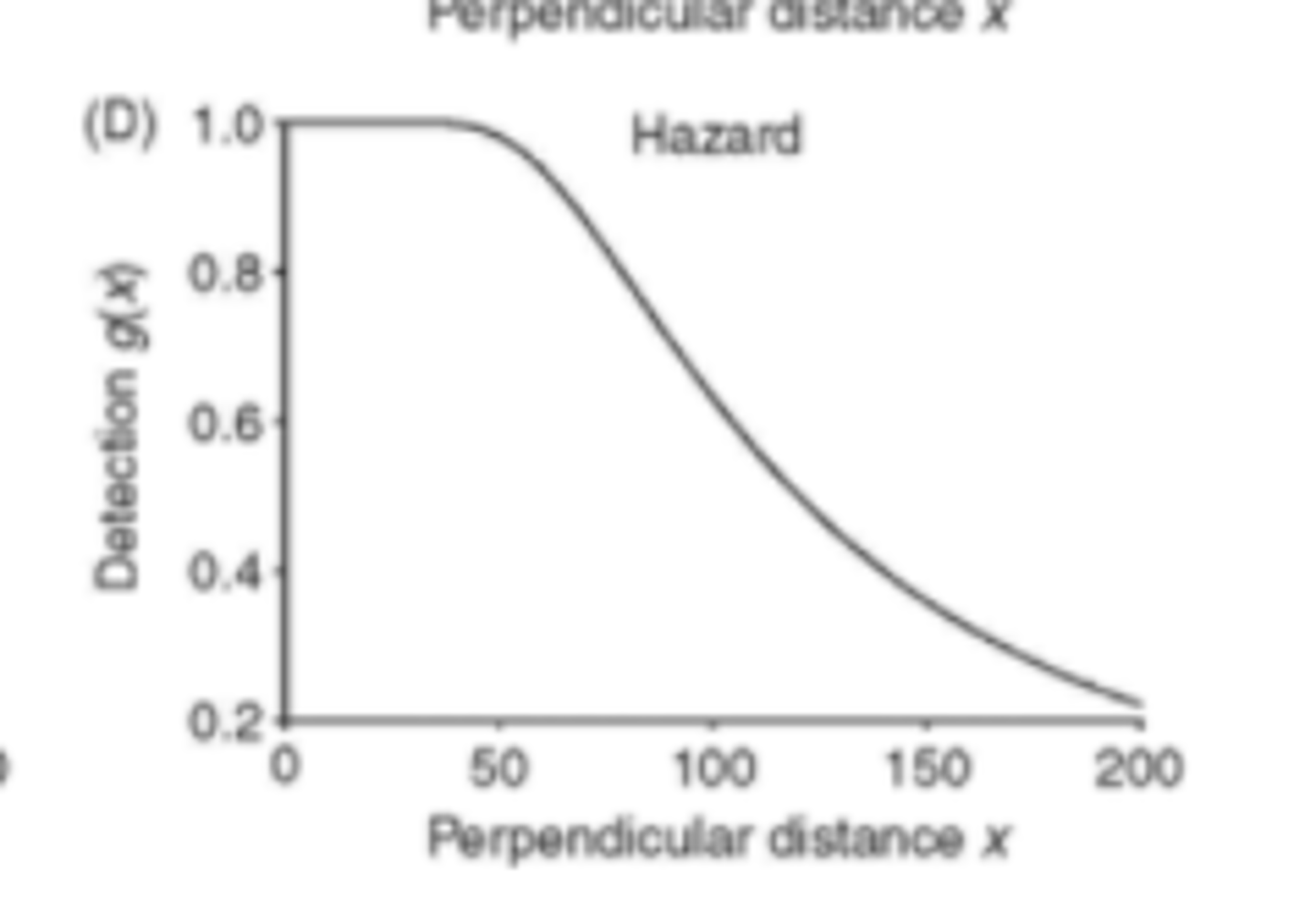
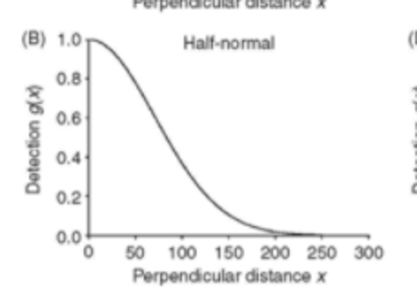
Hazard detection graph

Uniform detection graph

Negative exponential detection graph

Half-normal detection graph

Pros and cons of line transects

-mammals

-larger areas quicker

-distance estimation while moving may be difficult

Pros and cons of point counts

-birds

-more practical in rough terrain

-fixed time

-more time to see or hear

-less area covered

Sampling principles

-objective

-target population

-sampling units

Cormack-Jolly-Seber (CJS) Model

-Apparent survival

-Capture probability

-Cannot estimate N

What is apparent survival

Cannot differentiate death from emigration

Jolly-Seber (JS) Model

-Estimation of survival AND recruitment

-Can estimate N with strong assumptions, but still difficult

Pollock's Robust Design Model

-Combines closed and open models, N, survival, and recruitment

-Flexible

What are the three open population models?

Cormack-Jolly-Seber, Jolly-Seber, Pollock's Robust Design

Cormack-Jolly-Seber Assumptions

-Capture and survival probabilities for marked animals are the same

-Instantaneous recapture and release of animals

-All emigration from the study area is permanent

Dead recovery parameters

s - survival probability

f - probability of tag recovery

What kind of survival can we get from telemetry studies

absolute survival

What can telemetry studies tell you for habitat

resource selection, home range estimation, movements and activity patterns

What can telemetry studies tell you about survival

known fate and Kaplan-Meier approaches, little detection error

Binomial models with "known fate" assumptions

-The fates of animals are known

-Fates are independent of eachother

Violations of binomial "known fate" models

Technological error, hunting, herding behavior

Censored Individuals

unknown what happened to the individual, left the capture site

Kaplan-Meier model

-allows for "known fates" and censoring

-allows for staggered entry

How to calculate population in the Kaplan-Meier model

Population = number of individuals - censored - dead

Issues with the life table analysis

-not actually estimating true population size

-dont know how many animals are in each age class

-assuming distribution is stable

-age classes can be targeted differently

Abundance vs. Occupancy

-Data to estimate abundance can be difficult to collect

-Obtaining occupancy data is usually less intensive and cheaper

Population level state variables

Abundance and density

Vital rates: survival and recruitment

Landscape level state variables

Patch occupancy of a single species

Vital rates: patch colonization and extinction

Community level state variables

Species richness, patch occupancy of multiple species

Vital rates: patch colonization and extinction of multiple species

What does absence data tell us

This species does not occur at the particular site or was not detected by the investigator

Site occupancy information uses

-Surveys of geographic range

-Habitat relationships

-Interspecific interactions

-Observed colonization and extinction

-Large scale monitoring programs

-Epidemiology

Site occupancy information problems

-Estimates what fraction of sites is occupied by a species

-Species are not always detected, even when present

Site occupancy information solutions

Replication

Temporal replication

repeat visits to sample units

Spatial replication

randomly selected 'sites' or sample units within area of interest

Naive occupancy

Species present detected at least once in all the total sites surveyed

Probabilistic Model Assumptions

-Sites are closed to changes in the occupancy state between sampling

-No heterogeneity that cannot be explained by covariates

-The detection process is independent at each site

-Species identifies correctly

Occupancy study design

-selecting sampling units

-season (breeding, migration, etc...)

-repeat surveys

Primary sampling seasons

Long intervals between sampling periods, occupancy can change

Secondary sampling periods

Short intervals between periods, occupancy not expected to change

Dynamic occupancy model assumptions

-no heterogeneity that cannot be explained by covariates

-the detected process is independent at each site

-species are IDed correctly

-no colonization and extinction between secondary periods

-no unmodeled heterogeneity in colonization or extinction between primary periods