4A10 flow instability
1/63
There's no tags or description
Looks like no tags are added yet.
Name | Mastery | Learn | Test | Matching | Spaced | Call with Kai |
|---|
No analytics yet
Send a link to your students to track their progress
64 Terms
Defining pertubations for flow instability
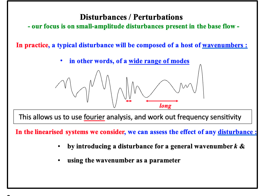
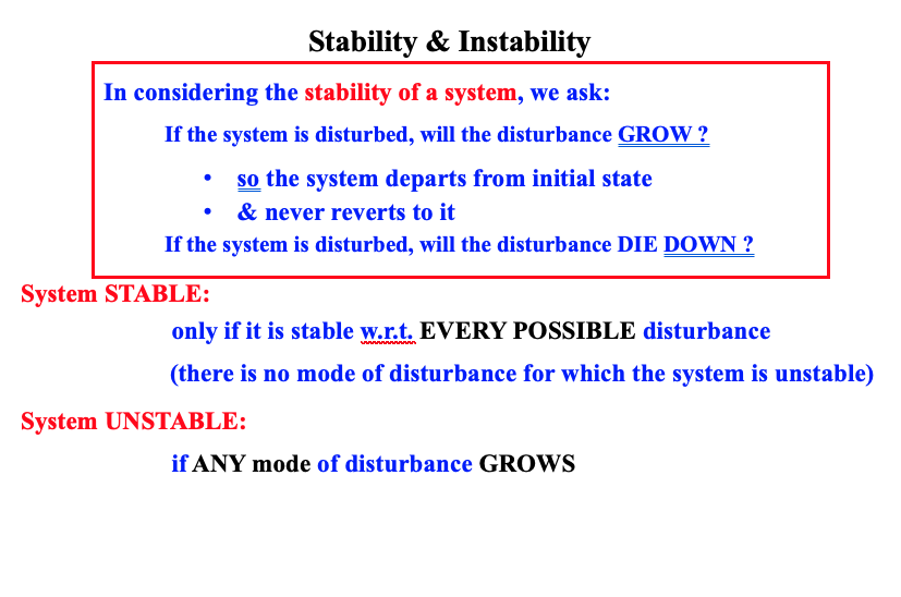
What is stability
Every single frequecny and mode of pertubation that we input needs to be stable for stability.
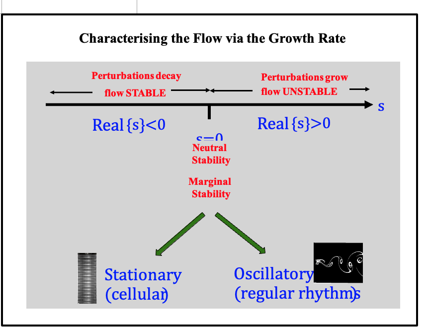
can characterise this with a laplace transform and teh value of s
Marginal stability
WE can also have marginal stability situations
stationary basically standing wave solutions
oscillatory rhyrthms
Methods of analysing stability.
We have two ways of analysing stability:
Linerarised equations
looking at small pertubations
solve for the growth rate
Energy analysis
see if energy is released or needed for a given pertubation
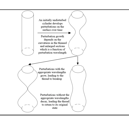
Break up of liquid jet: Setup and background
Here we’re trying to find the critical reynolds number for a liquid jet:
the physical mechanism is surface tension resulting in varying energy differences.
There is a squeeze from a smaller curvature increasing surface tension, balanced out by length wise curvature to some extent
we will work out an energy argument based on surface tension
Using conservation of volume to link how our curvatures in both directions
To work out growth rate:
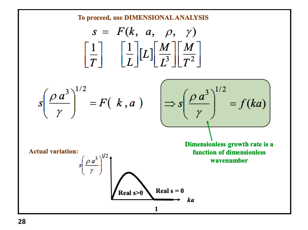
We will use a different method of using dimensional analysis to figure out the form of our growth rate equation
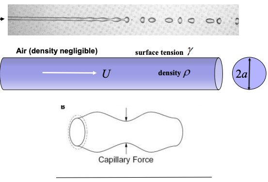
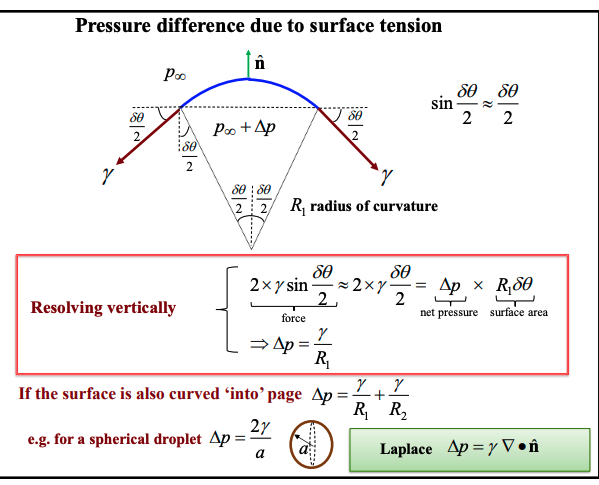
Break up of liquid jet: (note on surface tension)
Our surface tension can be defined in two ways:
Tension (N/m) basically a force per unit length, a pull on the fluid
Energy (J/m²) as a surface energy per unit area
To work out the pressure different due to surface tension
This is identical to a hoop stress derivation
So ΔP = γ/R for a single curvature (γ = ΔP/R)
and ΔP = 2γ/R for spherical (γ = ΔP/2R)
And for compound curvature. Δp=γ(R11+R21)
We are just balancing and integrating our pressure force (can take as a sector) with our surface tension at an angle. The trig terms will cancel out.
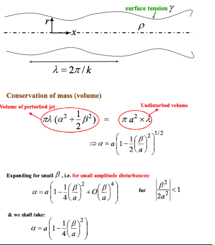
Break up of liquid jet: applying pertubation and considering volume
We will apply a small amplitude harmonic disturbance
r=α+βcoskx
Working out how α and β vary, given that we know the overall volume is constant
new volume is ∫0λπr2dx=∫0λπ(α+βcoskx)2dx=πλ(α2+21β2)
so:
Volume of perturbed jetπλ(α2+21β2)=Undisturbed volumeπa2×λ
⇒α=a(1−21(aβ)2)1/2
small amplitude:
β is much smaller the α, so can rewrite this as a binomial expansion
α=a(1−41(aβ)2)
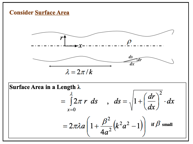
Break up of liquid jet: considering surface area
Our surface tension is an energy per unit area
To work out stability, we basically want to see if our pertubation increase or decreases the area
this will tell us if the energy increase or decreases
Using the constraint from before, we can use this to work out the surface area. The result is shown in the picture
Detailed maths
Transform coordinate system along length to dx
=∫x=0λ2πrds,ds=1+(dxdr)2⋅dx
now subbing in our expression for r both in 2πr and dr/dx
ds=dx(1+(βksinkx)2)1/2 taking an expansion as β is really small:
=dx(1+21β2k2sin2kx+O(βk)4)
Now subbing in the integral
S.A.=2π∫0λ(α+βcoskx)(1+21β2k2sin2kx)dx
quite easy to solve, basically in terms of chain rule if we get into the form sin(cos)^n or cos(sin)^n
this results in:
=2πλ(α+41αβ2k2)
now subbing in our expression for α
α=a(1−41(aβ)2+o(aβ)4)
=2πλa(1+4β2(k2−a21))
=2πλa(1+4a2β2(k2a2−1))if β small
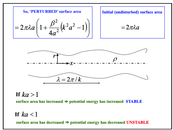
Break up of liquid jet: stability result
Stability criteria can be seen in the image.
With small β we can basically consider this as a balance of curvature
At long wavelengths we get an increase in curvature from the radius change (aximuthal) resulting in instability
But this is counteracted by some negative curvature from the axial curvature
at the balance these basically cancel each other out.
Break up of liquid jet: growth rate.
Here we are considering dimensional analysis: If we consider a perturbation in the form:
r=a+estβcoskx
Our growth rate s has dimensions 1/T, this depends on
wavenumber (1/L)
original radius (a)
density (M/L³)
surface tension (M/T²)
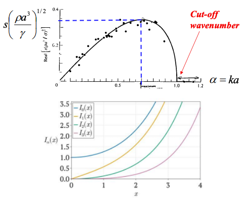
we get s(γρa3)1/2=f(ka)
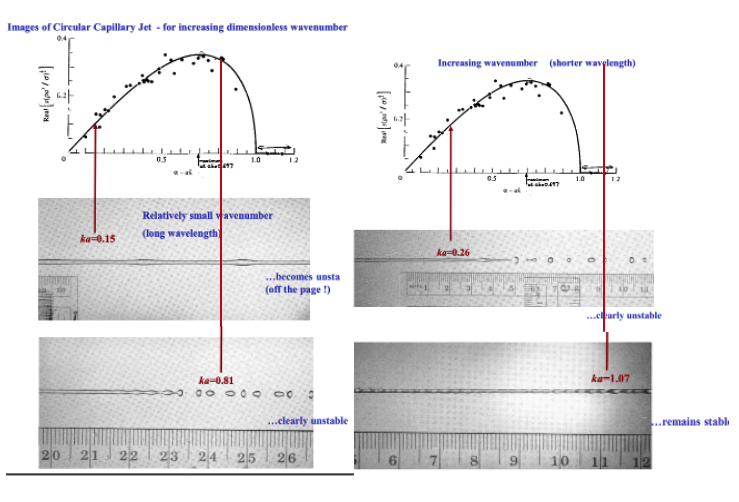
real variation
our actual variation in this non dimensionalised form can be seen below.
Break up of jet : limitations in analysis
effect of gravity
we have ignored gravity so far, we can examine this effect by comparing the hydrostatic pressure difference to the surface tension pressure difference
Hydrostatic pressure difference: Δp∼ρga
Surface tension pressure diffference: Δp∼γ/a
So our metric for whether this is significant is by dividing these 2
ρga≪aγ⟹a≪ρgγ
cannot predict drop size bc this is large disturbance
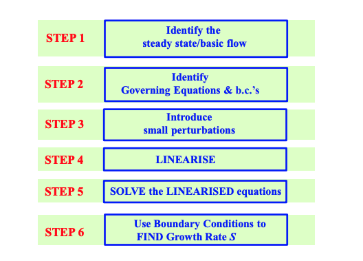
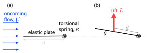
Basic recipe for linear analysis.
we have 6 basic steps for linear stability analysis.
1: Identify steady flow
We want a solution for our unperturbed flow, generally want:
Velocity U(x), Pressure P(x), and Interface position η
2: Identify governing equations/boundary counditions
Governing equations like navier stokes and continuity, boundary condition like no slip, pressure at boundary etc.
3: Introduce small pertubations about the flow
Add small pertubations to every variable:
u(x,t)=U(x)+u′(x,t)
p(x,t)=P(x)+p′(x,t)
η(x,t)=a(x)+η′(x,t)
4: linearise governing equations
Express our governing equations in terms of these pertubations
Remember our pertubations are small so we can neglect their products (similar to boundary layer equations)
allows us to remove many terms
5: solve linearised equations of motion
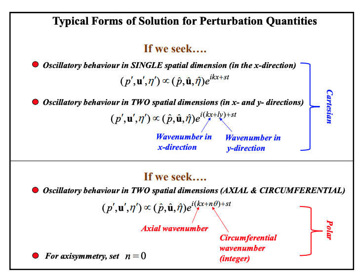
Generally we want normal mode exponential solutions
eg: u′(x,z,t)∝u^(z)eikx+st (shape term and then wave evolution term)
This is a separation of variables approach
6: use boundary conditions and find S
If s is on RHP then it is unstable
Why this is useful
any disturbance can be expressed as a fourier series
can look at the frequency component sensitivity
we need every frequency to be stable for stability
Typical form of linear stability modal solutions
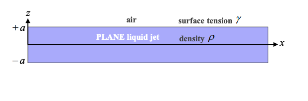
Linear stability analysis for plane jet: setup and introduction
Here we are considering a plane (not circular jet) so degrees of freedom (x,z,t)
We will following our linear analysis recipe to solve this:
We will look at the interface position η, pressure p and velocity U
Our flow is governed by continuity and the euler equation (inviscid navier stokes)
We have a pressure boundary condition on the surface, dependent on surface tension, as well as a kinematic boundary condition (fluid particles on surface stay on surface)
Goal here is to try eliminate variables
We will combine euler and continuity together to a single governing euqation
We get a second equation by subbing into the boundary conditions and combining togther
combine equations together to get a final PDE
Now solve PDE with separation of variables with a Modal solution
Use our boundary condition that we know this is solve for Z=a
work out growth rate.
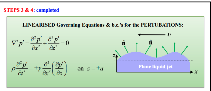
Linear stability analysis for plane jet: Governing equations and boundary conditions
We have two governing equations for this scenario:
∇⋅u=0 (mass conservation)
∂t∂u+(u⋅∇)u=−ρ1∇p (inviscid momentum equation)
We also have two boundary conditions:
Pressure boundary condition
Our pressure on interface equals atmospheric pressure + a surface tension term
This is p−p∞=γ∇⋅n^on z=η(x,t)
n^=∣∇F∣∇F, where F=0 is the equation defining the surface.
Kinematic boundary condition
this is basically stating particles on the surface must remain on the surface, basically our material derivative on the surface must be zero.
Our surface function is F(x,z,t)=z−η(x,t)=0 .
So: DtDF=[∂t∂F+(u⋅∇)F]=0
∂t∂F=−∂t∂η
(u⋅∇)F=u∂x∂F+v∂y∂F+w∂z∂F=−u∂x∂η+0+w(1)
so we get ∂t∂η+u∂x∂η=w on z=η(x,t) (w is the vertical velocity)
![<p>We have two governing equations for this scenario:</p><ul><li><p>$$\nabla \cdot \mathbf{u} = 0$$ (mass conservation)</p></li><li><p>$$\frac{\partial \mathbf{u}}{\partial t} + (\mathbf{u} \cdot \nabla)\mathbf{u} = -\frac{1}{\rho}\nabla p$$ (inviscid momentum equation)</p></li></ul><p></p><p>We also have two boundary conditions:</p><p><strong>Pressure boundary condition</strong></p><ul><li><p>Our pressure on interface equals atmospheric pressure + a surface tension term</p></li></ul><p>This is $$p - p_{\infty} = \gamma \nabla \cdot \mathbf{\hat{n}} \quad \text{on } z = \eta(x,t)$$</p><p>$$\mathbf{\hat{n}} = \frac{\nabla F}{|\nabla F|}$$, where $$F = 0$$ is the equation defining the surface.</p><p></p><p><strong>Kinematic boundary condition</strong></p><p>this is basically stating particles on the surface must remain on the surface, basically our material derivative on the surface must be zero.</p><p>Our surface function is $$F(x, z, t) = z - \eta(x, t) = 0$$ .</p><p>So: $$\frac{DF}{Dt} = \left[ \frac{\partial F}{\partial t} + (\mathbf{u} \cdot \nabla)F \right] = 0$$</p><ul><li><p>$$\frac{\partial F}{\partial t} = -\frac{\partial \eta}{\partial t}$$</p></li><li><p>$$(\mathbf{u} \cdot \nabla)F = u\frac{\partial F}{\partial x} + v\frac{\partial F}{\partial y} + w\frac{\partial F}{\partial z} = -u\frac{\partial \eta}{\partial x} + 0 + w(1)$$</p></li></ul><p></p><p>so we get $$\frac{\partial\eta}{\partial t}+u\frac{\partial\eta}{\partial x}=w\text{ on }z=\eta(x,t)$$ (w is the vertical velocity)</p><p></p>](https://assets.knowt.com/user-attachments/a3a6c2d0-7a7b-4ada-9ec5-5cac33bdc313.png)
Linear stability analysis for plane jet: Adding pertubations and finding governing PDE
Basically our goal is to sub in all our values and then simplify so we get a single PDE
Introducing perturbations:
We are adding perturbations in all three variables (base velocity of zero from reference frame change)
Velocity: u=0+u′(x,z,t)⟹u=u′
Pressure: p=P+p′(x,z,t)⟹p=p∞+p′
Interface: η=a+η′(x,t)
Overview of equations
Our governing equations are:
∇⋅u=0 (mass conservation)
∂t∂u+(u⋅∇)u=−ρ1∇p (inviscid momentum equation)
And boundary conditions are:
p−p∞=γ∇⋅n^on z=η(x,t)
∂t∂η+u∂x∂η=∂t∂z
subbing in to remove governing equations
Continuity: ∇⋅u′=0
Euler: ∂t∂u′+product of small terms(u′⋅∇)u′=−ρ1∇(P+p′)
ρ∂t∂u′=−∇p′ (remember this is a VECTOR equation)
Combining both equations by taking the divergence of both sides, we get a laplacian equation:
∇2p′=∂x2∂2p′+∂z2∂2p′=0
subbing into the pressure boundary condition
p−p∞=γ∇⋅n^
finding unit normal
n^=∣∇F∣∇F=(∂x∂η′)2+(0)2+(1)2−∂x∂η′i+0j+k≈−∂x∂η′i+0j+k (neglect squared term at bottom)
This is basically just our gradient as maybe expected, as our vector does not need to be normalised due to small movements
our pressure is
∂t∂η′=w′on z=a
p′=−γ∂x2∂2η′on z=a
subbing into kinematic boundary condition
∂t∂η+u∂x∂η=won z=η(x,t)
we get:
∂t∂η′=w′on z=a (once we neglect small terms)
combining boundary conditions
We can combine to eliminate η
differentiating pressure twice to get ∂t∂η′
∂t2∂2p′=−γ∂x2∂2(∂t2∂2η′) now we sub in our z velocity
∂t2∂2p′=−γ∂x2∂2(∂t∂w′) now we use the Z component of our combined euler equation
ρ∂t∂u′=−∇p′ , Z component is ρ∂t∂w′=−∂z∂p′
combined we get
∂t2∂2p′=−γ∂x2∂2(−ρ1∂z∂p′)
boundary equation PDE
rearranging this our final PDE is:
ρ∂t2∂2p′=γ∂x2∂2(∂z∂p′)on z=a
Linear stability analysis for plane jet: Finding solutions for PDE
We’re looking for normal mode solutions, (basically doing separation of variables)
p′(x,z,t)=p^(z)eikx+st
Now plugging this into the governing equation first (laplace equation):
∇2p′=0.
dz2d2p^(z)−k2p^(z)=0 this reduces it down to an ODE
this has a hyperbolic solution:
p^(z)=Ae−kz+Be+kzfor constants A and B
We clearly have symmetry about Z, so the constants must be the same
So our perturbation is in the form: p′=A(e−kz+e+kz)eikx+st
to find growth rate we sub into boundary condition
ρ∂t2∂2p′=γ∂x2∂2(∂z∂p′)on z=a
ρs2A(eka+e−ka)eikx+stz=a=γ∂x2∂2[kA(ekz−e−kz)eikx+st]z=a
ρs2A(eka+e−ka)=γ(−k2)[kA(eka−e−ka)] can eliminate A and this is a tanh equation
s2=−ρa3γ(ka)3tanh(ka)
verdict
Tanh is positive for all positive values of ka
so s² = -ve
so s must be purely imaginary neutrally stable
makes sense if we just think about the energies for 2 seconds, clearly our areas stay the same
Result from dimensional analysis
s(γρa3)1/2=f(ka)ors2(γρa3)=F(ka)
matches form of s2=−ρa3γ(ka)3tanh(ka)
Linear stability analysis for circular jet: Growth rate
As we know for energy analysis this is unstable
Linear analysis tells us our growth rate (wiith very complicated maths)
s2=ρa3γIn(α)In′(α)α(1−α2−n2)where α=ka
Our In are modified bessel functions of the first kind, basically like our hyperbolic functions but for radially varying systems.
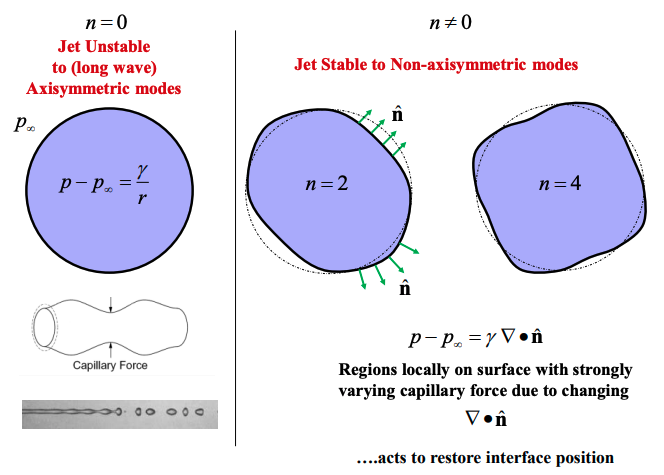
Linear stability analysis for circular jet: Modes
Only unstable for long wave axisymmetric modes
Stable for azimuthal modes, strongly varying capillary force restore interface position.
Axisymmetric n = 0
s2=ρa3γIn(α)In′(α)α(1−α2−n2)where α=ka (1−α2−n2)
then (1-α²) is positive if α (ka) < 1
Azimuthal n ≠ 0
We have a boundary condition on n, so it must take integer values due to the rotation symmetry
immediately this results in (1−α2−n2) being negative
this results in a stable jet.
We can see these modes on the right
Linear stability analysis for circular jet: Development of pertubations
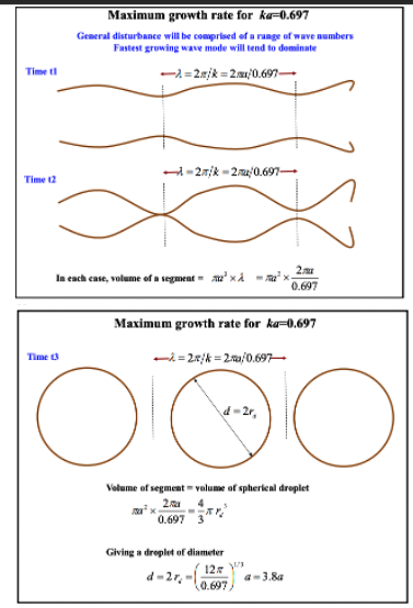
Linear stability analysis for circular jet: Droplet size predictions
Although linear analysis isn’t really meant for this, because it considers small pertubations, we can perform a surprisingly accurate estimation for the droplet size.
Basically we take maximum growth wavelength (ka =0.697)
see the volume contained within that wavelength
this gives us d = 3.8a
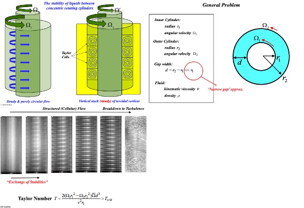
Taylor couette flow: overview
Two rotating cylinders with a “narrow gap”
This results in the formation of cells
This is an exchange of stability, as we go from one stable mode to another stable mode.
steps for solving
We will first look at the steady state
Taylor courette flow: Solving steady state base flow
Base flow
Here we are assuming a purely circular flow, so the flow is only in the Uθ direction, and this must only vary the radius.
Our flow structure is thus:
u(r)=radial0er+circumferentialUθ(r)eθ+vertical0ez
Solving for base flow structure
Our base flow is governed by two governing equations, navier stokes and continuity, writing these out in cylindrical coordinates we get:
Navier stokes
Radial: ∂t∂ur+(u⋅∇)ur−ruθ2=−ρ1∂r∂p+ν[∇2ur−r2ur−r22∂θ∂uθ]
Circumferential: ∂t∂uθ+(u⋅∇)uθ+ruruθ=−ρr1∂θ∂p+ν[∇2uθ+r22∂θ∂ur−r2uθ]
Vertical: ∂t∂uz+(u⋅∇)uz=−ρ1∂z∂p+ν[∇2uz]
Continuity this is the vector equation:
∇⋅u=r1∂r∂(rur)+r1∂θ∂(uθ)+∂z∂(uz)=0
Plugging in our solutions to simplify
We can simplify given that U is only in the circumferential direction, and only varies with θ.
Continuity: Automatically satisfied by our flow assumptions, every term is zero
Radial: −ruθ2=−ρ1∂r∂p
Circumferential: ∂t∂uθ=ν[∂r2∂2uθ+r1∂r∂uθ−r2uθ]
(splitting laplacian), pressure must be constant since its periodic
Vertical: 0=−ρ1∂z∂p No vertical pressure gradient
Now for steady flow
dr2d2uθ+r1drduθ−r2uθ=0
Solving ODE and adding boundary conditions
Use the substitution r=ex for Euler-Cauchy equation so x=ln(r)
For first derivative:
drdUθ=dxdUθdrdx=dxdUθ(r1)
⟹rdrdUθ=dxdUθ
For second derivative:
dr2d2Uθ=drd(drdUθ)=drd(r1dxdUθ) (now use product rule)
dr2d2Uθ=drd(r1dxdUθ)=r21(dx2d2Uθ−dxdUθ)
Plugging back together we get:
r21((dx2d2Uθ−dxdUθ)+(dxdUθ)−Uθ)=0
dx2d2Uθ−Uθ=0
result
This is solved with:
Uθ=Aex+Be−x
Giving us a solution of:
Uθ(r)=Ar+rB
we just apply no slip condition to give A and B
A=r22−r12Ω2r22−Ω1r12
B=r22−r12(Ω1−Ω2)r12r22
Taylor courette flow: Physical reason for instability:
Above a critical Taylor number (1708) our system becomes unstable. This is defined as: T = \frac{2(\Omega_1 r_1^2 - \Omega_2 r_2^2)\overline{\Omega}d^3}{\nu^2 r_1} > T_{\text{crit}} \approx 1708
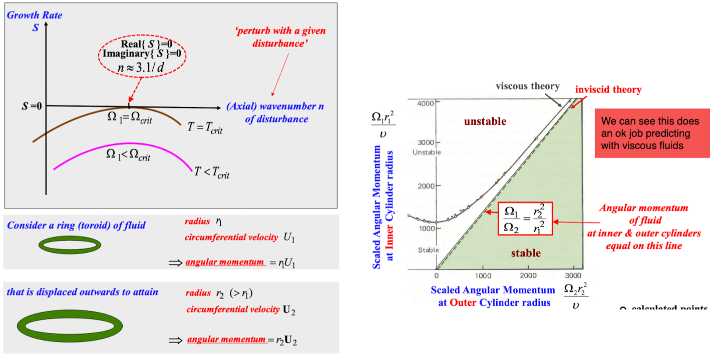
We can see how on the graph, our growth rate curve increases with increasing taylor number, and how we only get marginal growth at the critical taylor number.
at even higher taylor numbers, our flow changes wave number
Physical explanation
The physical explanation here is pretty much identical to a ball on a spring which is spun around.
Angular momentum
If we consider a toroid of fluid with radius r₁ and velocity U₁ , it’s angular momentum is r₁U₁
Now if this is displaced slightly it must conserve angular momentum, with radius r₂ and U₂
The velocity decreases with: U2′=(r2r1)U1
The velocity decrease but we don’t know if this is enough to stay within our centripetal force boudary
Centripetal force:
Now at equilibrium our force holding the fluid in place is centripetal force.
−ρ1∂r∂p=−r2U22 at r₂
If we perturb our fluid from U₁ , and the resulting U₂’ is LOWER than U₂, then our system is stable.
Finding stability criteria
At our boundary, our perturbation will result in U₂’ = U₂
So setting this equal we get:
(r2r1U1)2≤U22⟹(r1U1)2≤(r2U2)2
(r22Ω2)2−(r12Ω1)2≥0
this means our angular momentum must INCREASE with RADIUS for stability
this is an inviscid prediction which matches well at high speeds.
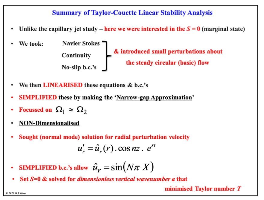
Taylor courette flow: Linear stability analysis
Here we’re doing our same 6 step process:
we want to find the marginal stability state for when the flow regime switches
Setting up system and plugging in pertubations
Same with our base equations of navier stokes and continuity
Our perturbations are:
p=P(r)+p′(r,z,t)
uθ=Uθ+uθ′(r,z,t)
uz=0+uz′(r,z,t)
ur=0+ur′(r,z,t)
Plugging this into our cylindrical navier stokes and continuity, eliminating products of small terms, we get:
Radial: ∂t∂ur′−2rUθuθ′=−ρ1∂r∂p′+ν(∇2ur′−r2ur′)
Circumferential: ∂t∂uθ′+ur′drdUθ+rur′Uθ=ν(∇2uθ′−r2uθ′)
Vertical: ∂t∂uz′=−ρ1∂z∂p′+ν(∇2uz′)
Continuity: rur′+∂r∂ur′+∂z∂uz′=0
Narrow gap approximation
we can further simplify our equations with a narrow gap approximation.
Basically curvature is identical on both faces
any gradients which are order X/d so any derivatives with respect to r generally, much bigger than say a u/r term
Our equations are now: (also moving our operators together)
Radial: (∂t∂−ν∇~2)ur′−(r2Uθ)uθ′=−ρ1∂r∂p′
Circumferential: (∂t∂−ν∇~2)uθ′+(2A)ur′=0
A is our base flow term, since we ur′(drdUθ+rUθ)
So can plug in drdUθ=A−r2B and rUθ=A+r2B
Vertical:
(∂t∂−ν∇~2)uz′=−ρ1∂z∂p′
Finding our PDE
now our goal from our narrow gap equations
Remove pressure term in radial equation using vertical equation
∂z2∂2(Radial Eq. 1)−∂z∂∂r∂(Vertical Eq. 2)
use continuity to remove the the Uz term
This gives us two PDEs in just ur and uθ
(∂t∂−ν∇~2)∇~2ur′=(r2Uθ)∂z2∂2uθ′
(∂t∂−ν∇~2)uθ′+(2A)ur′=0
Solving PDE
we’re using normal mode solutions (separation of variables) to find the solution
ur′=Unknown radialu^r(r)⋅From observationcos(nz)⋅Growth rateest
uθ′=u^θ(r)⋅cos(nz)⋅est
This results in two ODEs
[ν(dr2d2−n2)−S]u^θ=2A⋅u^r
[ν(dr2d2−n2)−S][dr2d2−n2]u^r=(r2Uθn2)u^θ
We can note that our constant for the second equation is not constant
similar rotation approximation
If our rotation is similar though, our base flow circular velocity doesn’t really vary. so can do
rUθ=Ω=21(Ω1+Ω2)
This gives us:
[ν(dr2d2−n2)−S][dr2d2−n2]u^r=(r2Uθn2)u^θ
and if we use equation 3 to get rid of uθ
[ν(dr2d2−n2)−S]2[dr2d2−n2]u^r=(4Ωn2A)u^r
this is an ODE in just R. Our growth rate S drops out
Boundary conditions:
Now to find boundary conditions we have
No flow through cylinder walls: u^r=0at r=r1,r2
No slip on walls u^z=0at r=r1,r2 so also ∂z∂uz′=0
Continuity: As ∂r∂ur′+∂z∂uz′=0 ∴ drdu^r=0at r=r1,r2
Also u^θ′=0
Now subbing this into our ODE equation, we can get an equation value at r = r₁ and r₂
[ν(dr2d2−n2)−S][dr2d2−n2]u^r=(r2Uθn2)u^θ
no Uθ so right hand size gets removed
we get:
dr4d4u^r−(2n2+νS)dr2d2u^r=0on r=(r1,r2) (this is our 6th boundary condition)
this is because our equation for Uᵣ is 6th order
so we need 6 boundary conditions for uᵣ, 3 on each wall.
Solving ODE
Our system is now:
ODE:
[ν(dr2d2−n2)−S]2[dr2d2−n2]u^r=(4Ωn2A)u^r
6 boundary conditions at r = r₁ and r₂
u^r=0:
drdu^r=0
dr4d4u^r−(2n2+νS)dr2d2u^r=0
Non dimensionalise
Defining two variables to non dimensionlise our lengths
X=dr−r1 so X = 0 at inner gap and X = 1 at outer gap
Axial wavenumber: a=nd
This results in the ODE: below with the same boundary conditions:
(dX2d2−a2)3u^r=−T⋅(a2)u^r where the taylor number T=ν2r12(Ω1r12−Ω2r22)Ωd3≈viscosityinertia
This is extremely hard to solve
Boundary condition simplification
if we simplify the boundary condition dr4d4u^r−(2n2+νS)dr2d2u^r=0on r=(r1,r2)
to dr4d4u^r=0
Now we just end up with a sinusoidal solution:
u^r=sin(NπX)where N=1,2,3… (Equation 7)
this gives us a critical taylor number of 658
this is compared to the actual value of 1708 without the simplified boundary conditions
This is when we set the wave number to 1
Result structure
With our unsimplified structure, we find our critical wavelength by finding the minimum of the taylor number vs wave number curve, for N = 1
we can note in our critical solution where a = 3.1, we can almost square cells as 3.1 is basically π
![<p>Here we’re doing our same 6 step process:</p><p>we want to find the marginal stability state for when the flow regime switches</p><p></p><h4 id="eabb9d0b-ea6f-4cd3-ba91-207d150aafa6" data-toc-id="eabb9d0b-ea6f-4cd3-ba91-207d150aafa6" collapsed="false" seolevelmigrated="true">Setting up system and plugging in pertubations</h4><ul><li><p>Same with our base equations of navier stokes and continuity</p></li></ul><p></p><p>Our perturbations are:</p><ul><li><p>$$p = P(r) + p'(r, z, t)$$</p></li><li><p>$$u_{\theta} = U_{\theta} + u_{\theta}'(r, z, t)$$</p></li><li><p>$$u_{z}=0+u_{z}^{\prime}(r,z,t)$$</p></li><li><p>$$u_r = 0 + u_r'(r, z, t)$$</p></li></ul><p></p><p>Plugging this into our cylindrical navier stokes and continuity, eliminating products of small terms, we get:</p><ul><li><p>Radial: $$\frac{\partial u_r'}{\partial t} - 2\frac{U_{\theta} u_{\theta}'}{r} = -\frac{1}{\rho}\frac{\partial p'}{\partial r} + \nu\left(\nabla^2 u_r' - \frac{u_r'}{r^2}\right)$$</p></li><li><p>Circumferential: $$\frac{\partial u_{\theta}'}{\partial t} + u_r' \frac{dU_{\theta}}{dr} + \frac{u_r' U_{\theta}}{r} = \nu\left(\nabla^2 u_{\theta}' - \frac{u_{\theta}'}{r^2}\right)$$</p></li><li><p>Vertical: $$\frac{\partial u_z'}{\partial t} = -\frac{1}{\rho}\frac{\partial p'}{\partial z} + \nu\left(\nabla^2 u_z'\right)$$</p></li><li><p>Continuity: $$\frac{u_r'}{r} + \frac{\partial u_r'}{\partial r} + \frac{\partial u_z'}{\partial z} = 0$$</p></li></ul><h4 id="880ec691-43f9-457b-a336-ab622896c0b4" data-toc-id="880ec691-43f9-457b-a336-ab622896c0b4" collapsed="false" seolevelmigrated="true">Narrow gap approximation</h4><p>we can further simplify our equations with a narrow gap approximation.</p><ul><li><p>Basically curvature is identical on both faces</p></li><li><p>any gradients which are order X/d so any derivatives with respect to r generally, much bigger than say a u/r term</p></li></ul><p>Our equations are now: (<strong>also moving our operators together)</strong></p><ul><li><p>Radial: $$\left(\frac{\partial}{\partial t}-\nu\tilde{\nabla}^2\right)u_{r}^{\prime}-\left(\frac{2 U_\theta}{r}\right)u_{\theta}^{\prime}=-\frac{1}{\rho}\frac{\partial p'}{\partial r}\text{ }$$</p></li><li><p>Circumferential: $$\left(\frac{\partial}{\partial t}-\nu\tilde{\nabla}^2\right)u_{\theta}^{\prime}+(2A)u_{r}^{\prime}=0\text{ }$$</p><ul><li><p>A is our base flow term, since we $$u_{r}^{\prime}\left(\frac{dU_{\theta}}{dr}+\frac{U_{\theta}}{r}\right)$$</p></li><li><p>So can plug in $$\frac{dU_{\theta}}{dr} = A - \frac{B}{r^2}$$ and $$\frac{U_{\theta}}{r} = A + \frac{B}{r^2}$$</p></li></ul></li><li><p>Vertical:</p><ul><li><p>$$\left(\frac{\partial}{\partial t}-\nu\tilde{\nabla}^2\right)u_{z}^{\prime}=-\frac{1}{\rho}\frac{\partial p'}{\partial z}$$</p></li></ul></li></ul><h4 id="aab7f9ec-d87b-484a-ab2f-bd2df65f14a1" data-toc-id="aab7f9ec-d87b-484a-ab2f-bd2df65f14a1" collapsed="false" seolevelmigrated="true">Finding our PDE</h4><p>now our goal from our narrow gap equations</p><ul><li><p>Remove pressure term in radial equation using vertical equation</p><ul><li><p>$$\frac{\partial^2}{\partial z^2}(\text{Radial Eq. 1}) - \frac{\partial}{\partial z}\frac{\partial}{\partial r}(\text{Vertical Eq. 2})$$</p></li></ul></li><li><p>use continuity to remove the the Uz term</p></li></ul><p></p><p>This gives us two PDEs in just $$u_r$$ and $$u_\theta$$</p><p>$$\left( \frac{\partial}{\partial t} - \nu \tilde{\nabla}^2 \right) \tilde{\nabla}^2 u_r' = \left( \frac{2U_\theta}{r} \right) \frac{\partial^2 u_\theta'}{\partial z^2}$$</p><p>$$\left( \frac{\partial}{\partial t} - \nu \tilde{\nabla}^2 \right) u_\theta' + (2A) u_r' = 0$$</p><p></p><h4 id="cc2d688f-6f5e-4bc9-8914-dc966e80ca0b" data-toc-id="cc2d688f-6f5e-4bc9-8914-dc966e80ca0b" collapsed="false" seolevelmigrated="true">Solving PDE</h4><p>we’re using normal mode solutions (separation of variables) to find the solution</p><ul><li><p>$$u_{r}^{\prime}=\underbrace{\hat{u}_{r}(r)}_{\text{Unknown radial}}\cdot\underbrace{\cos(nz)}_{\text{From observation}}\cdot\underbrace{e^{st}}_{\text{Growth rate}}$$</p></li></ul><ul><li><p>$$u_\theta' = \hat{u}_\theta(r) \cdot \cos(nz) \cdot e^{st}$$</p></li></ul><p></p><p>This results in two ODEs</p><ul><li><p>$$[\nu (\frac{d^2}{dr^2} - n^2) - S] \hat{u}_\theta = 2A \cdot \hat{u}_r$$</p></li><li><p>$$[\nu (\frac{d^2}{dr^2} - n^2) - S] [\frac{d^2}{dr^2} - n^2] \hat{u}_r = \left( \frac{2U_\theta n^2}{r} \right) \hat{u}_\theta$$</p></li></ul><p></p><p>We can note that our constant for the second equation is not constant</p><p><strong>similar rotation approximation</strong></p><p>If our rotation is similar though, our base flow circular velocity doesn’t really vary. so can do</p><ul><li><p>$$\frac{U_{\theta}}{r}=\overline{\Omega}=\frac{1}{2}(\Omega_1+\Omega_2)$$</p></li></ul><p></p><p>This gives us:</p><p>$$\left[ \nu \left( \frac{d^2}{dr^2} - n^2 \right) - S \right] \left[ \frac{d^2}{dr^2} - n^2 \right] \hat{u}_r = \left( \frac{2 U_\theta n^2}{r} \right) \hat{u}_\theta $$</p><p>and if we use equation 3 to get rid of $$u_{\theta}$$</p><p>$$\left[ \nu \left( \frac{d^2}{dr^2} - n^2 \right) - S \right]^2 \left[ \frac{d^2}{dr^2} - n^2 \right] \hat{u}_r = (4\overline{\Omega} n^2 A) \hat{u}_r$$</p><p>this is an ODE in just R. <strong>Our growth rate S drops out</strong></p><p></p><h4 id="3941080a-8f89-49dd-8206-f69863fcbebf" data-toc-id="3941080a-8f89-49dd-8206-f69863fcbebf" collapsed="false" seolevelmigrated="true">Boundary conditions:</h4><p>Now to find boundary conditions we have</p><ul><li><p>No flow through cylinder walls: $$\hat{u}_r = 0 \quad \text{at } r = r_1, r_2$$</p></li><li><p>No slip on walls $$\hat{u}_{z}=0\quad\text{at }r=r_1,r_2$$ so also $$\frac{\partial u_z'}{\partial z} = 0$$</p></li><li><p>Continuity: As $$\frac{\partial u_r'}{\partial r} + \frac{\partial u_z'}{\partial z} = 0$$ ∴ $$\frac{d\hat{u}_r}{dr} = 0 \quad \text{at } r = r_1, r_2$$</p></li><li><p>Also $$\hat{u}^{\prime}_{\theta}=0$$</p></li></ul><p></p><p>Now subbing this into our ODE equation, we can get an equation value at r = r₁ and r₂</p><p>$$\left[ \nu \left( \frac{d^2}{dr^2} - n^2 \right) - S \right] \left[ \frac{d^2}{dr^2} - n^2 \right] \hat{u}_r = \left( \frac{2U_\theta n^2}{r} \right) \hat{u}_\theta$$</p><ul><li><p>no Uθ so right hand size gets removed</p></li></ul><p>we get:</p><p>$$\frac{d^4 \hat{u}_r}{dr^4} - \left( 2n^2 + \frac{S}{\nu} \right) \frac{d^2 \hat{u}_r}{dr^2} = 0 \quad \text{on } r = (r_1, r_2)$$ (<strong>this is our 6th boundary condition)</strong></p><p><strong>this is because our equation for Uᵣ is 6th order</strong></p><p>so we need 6 boundary conditions for uᵣ, 3 on each wall.</p><p></p><h4 id="7f89ca69-cf05-43c7-a0fe-4211a4723383" data-toc-id="7f89ca69-cf05-43c7-a0fe-4211a4723383" collapsed="false" seolevelmigrated="true">Solving ODE</h4><p>Our system is now:</p><p><strong>ODE</strong>:</p><ul><li><p>$$\left[ \nu \left( \frac{d^2}{dr^2} - n^2 \right) - S \right]^2 \left[ \frac{d^2}{dr^2} - n^2 \right] \hat{u}_r = (4\overline{\Omega} n^2 A) \hat{u}_r$$</p></li></ul><p><strong>6 boundary conditions at r = r₁ and r₂</strong></p><ul><li><p><strong>$$\hat{u}_r = 0$$</strong>:</p></li><li><p>$$\frac{d\hat{u}_r}{dr} = 0$$</p></li><li><p>$$ \frac{d^4\hat{u}_{r}}{dr^4}-\left(2n^2+\frac{S}{\nu}\right)\frac{d^2\hat{u}_{r}}{dr^2}=0 $$</p></li></ul><p></p><p><strong>Non dimensionalise</strong></p><p>Defining two variables to non dimensionlise our lengths</p><ul><li><p>$$X = \frac{r - r_1}{d}$$ so X = 0 at inner gap and X = 1 at outer gap</p></li><li><p>Axial wavenumber: $$a = nd$$</p></li></ul><p></p><p>This results in the ODE: below with the same boundary conditions:</p><p>$$\left( \frac{d^2}{dX^2} - a^2 \right)^3 \hat{u}_r = -T \cdot (a^2) \hat{u}_r$$ where the taylor number $$T = \frac{2(\Omega_1 r_1^2 - \Omega_2 r_2^2)\overline{\Omega}d^3}{\nu^2 r_1} \approx \frac{\text{inertia}}{\text{viscosity}}$$</p><p>This <strong>is extremely hard to solve</strong></p><p></p><h4 id="a3b13477-59e7-4e30-8b6f-47f41cc605a6" data-toc-id="a3b13477-59e7-4e30-8b6f-47f41cc605a6" collapsed="false" seolevelmigrated="true">Boundary condition simplification</h4><p>if we simplify the boundary condition $$\frac{d^4 \hat{u}_r}{dr^4} - \left( 2n^2 + \frac{S}{\nu} \right) \frac{d^2 \hat{u}_r}{dr^2} = 0 \quad \text{on } r = (r_1, r_2)$$</p><p>to $$\frac{d^4 \hat{u}_r}{dr^4}=0$$ </p><p></p><p>Now we just end up with a sinusoidal solution:</p><p>$$\hat{u}_r = \sin(N\pi X) \quad \text{where } N = 1, 2, 3 \dots \text{ (Equation 7)}$$</p><p>this gives us a <strong>critical taylor number</strong> of <strong>658</strong></p><ul><li><p>this is compared to the actual value of <strong>1708 </strong>without the simplified boundary conditions</p></li><li><p>This is when we set the wave number to 1</p></li></ul><p></p><h4 id="f4e6519c-697e-41b7-b473-097f850fd1fb" data-toc-id="f4e6519c-697e-41b7-b473-097f850fd1fb" collapsed="false" seolevelmigrated="true">Result structure</h4><p>With our unsimplified structure, we find our critical wavelength by finding the minimum of the taylor number vs wave number curve, <strong>for N = 1</strong></p><ul><li><p>we can note in our critical solution where <strong>a = 3.1</strong>, we can almost square cells as 3.1 is basically π</p></li></ul><p></p>](https://assets.knowt.com/user-attachments/3b50a669-f8ff-474c-8811-b21d3ac91554.png)
Taylor courette flow: Overview of analysis
Where would we find shear flow instabilities
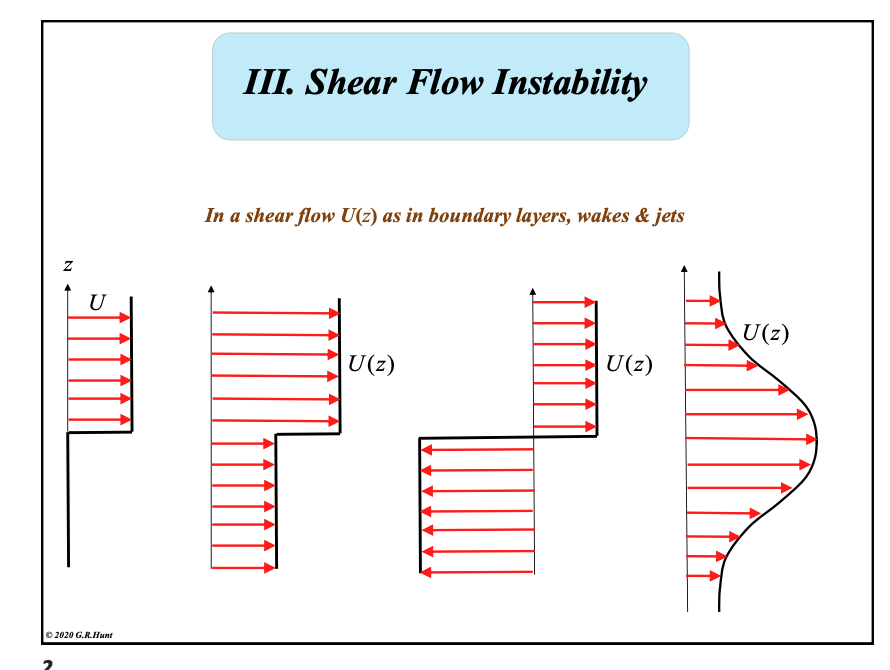
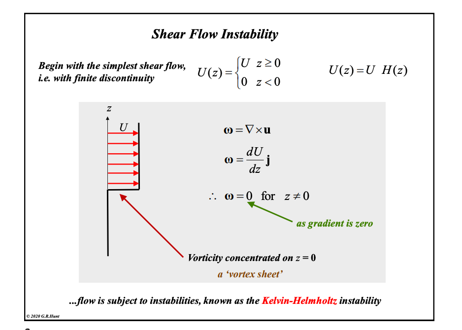
Vorticies in shear flow
If we have a finite discontinuity, this results in an infinitely thin vortex sheet
Examples of shear flow instabilities
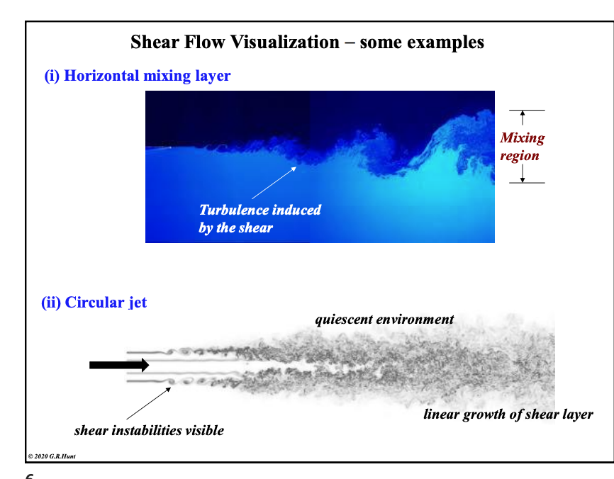
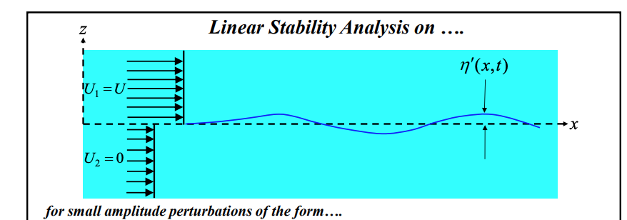
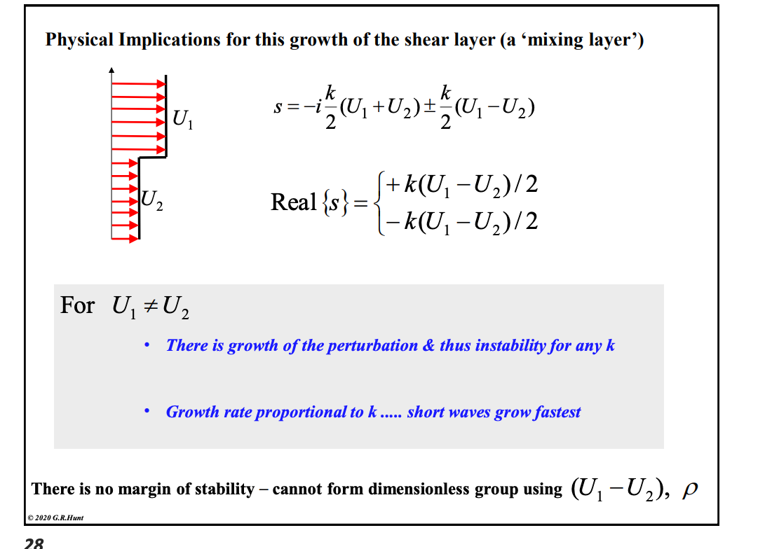
Solution for shear flow instabilities
If we apply a small pertubation to a boundary between fast moving and slow moving fluid
η′(x,t)=η^eikx+st
This gives us the solution where the growth mode is:
s=−i21kU±21kU
We have a pole on the right hand plane, this is unstable and oscillatory
if we write our our wave equation:
η′(x,t)=η^eik(x−21Ut)e21kUt
always unstable
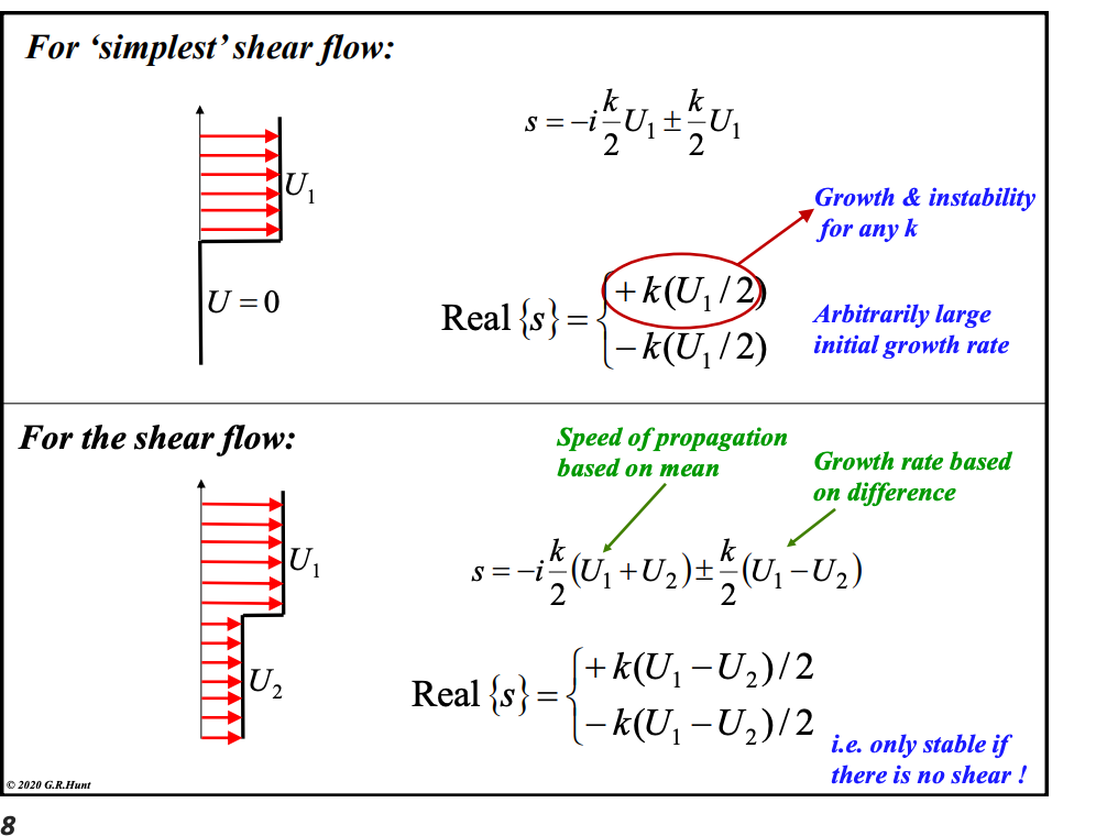
Dispersion relationship for shear flow instabilities
For our solution for the shear flow instability, we can write S in terms of the frequencies.
Our general solution is:
s=−i2k(U1+U2)±2k(U1−U2) (now subbing in s = -iw) for an a wave solution
ω=(21k(U1+U2))±i(21k(U1−U2))
We can note two things
The propagation component of our wave is equal to the mean of our two velocities: 21(U1+U2)
The growth component of our wave is equal to the difference of our two velocities: 21(U1−U2)
Only ever stable with no shear
further characteristisics of dispersion relation
Our dispersion relationship isn’t dispersive, our different wavelengths travel at the same speed
But it is distortive, as high wave numbers will grow much more quickly than small wave numbers
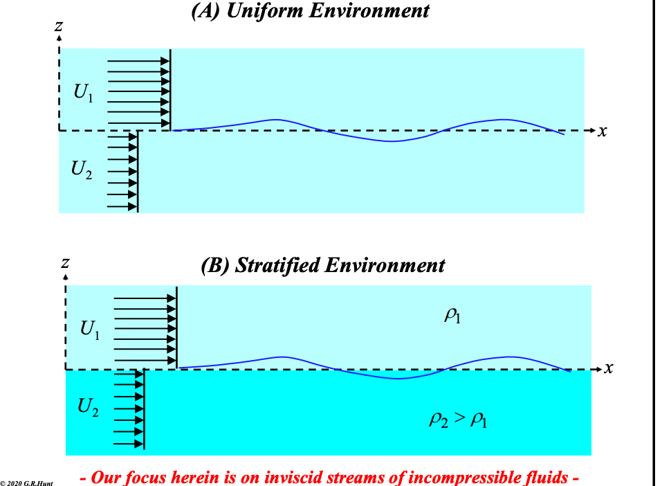
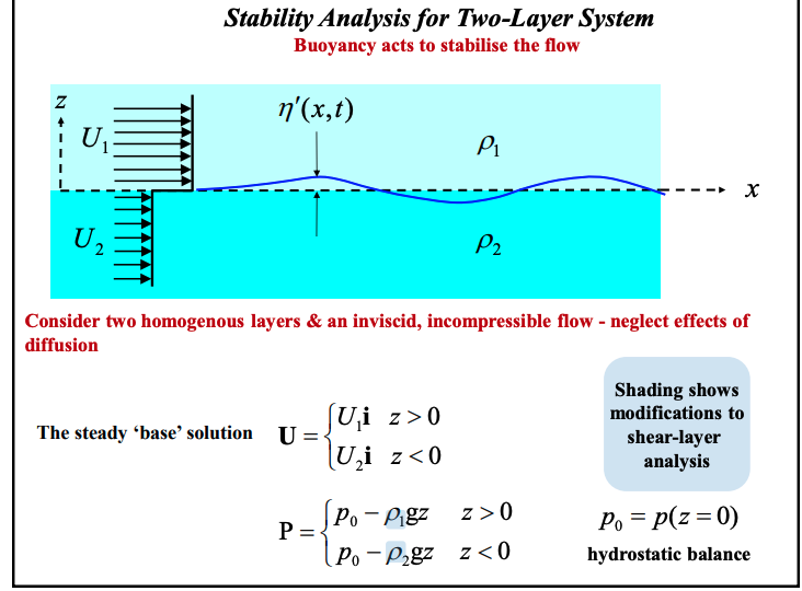
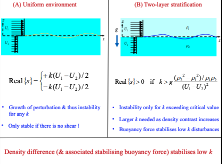
uniform vs stratified shear flow instability
stratified case has mechanism like bouyancy that can supress instability
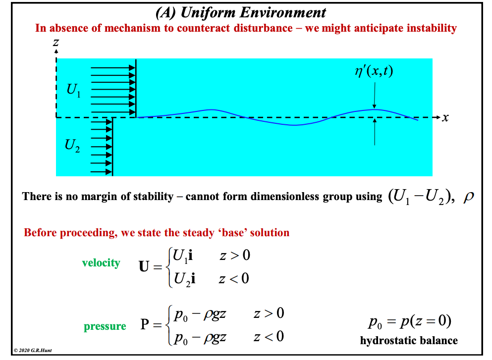
Shear flow linear analysis: base case
Our base case is shown below, where we have equal pressure at the interface but a discrete velocity jump:
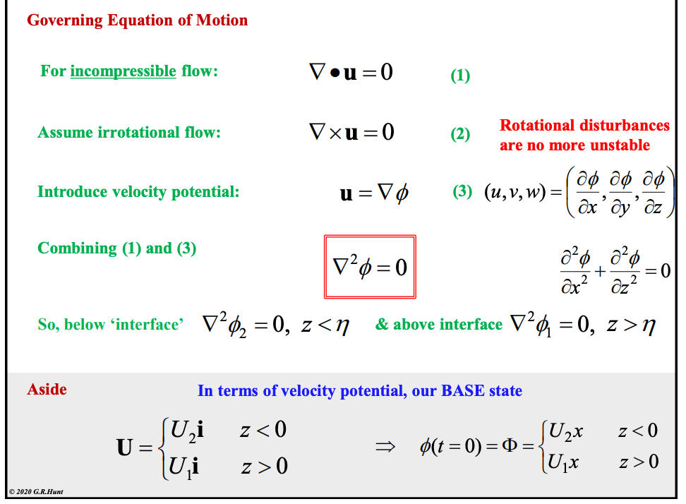
Shear flow linear analysis: governing equations:
We have an incompressible flow so have continuity expressed like this
Irrotational flow (shear is contained very locally)
define flow in terms of velocity potential, allowing for laplacian expression of velocity
Our flow is defined by our laplacian velocity potential above and below our interface
Shear flow linear analysis: boundary conditions
We have three boundary conditions
Pressure boundary condition: pressure must be the same across the interface
Kinematic boundary condition: Particles on interface must remain on interface
Localised disturbance: Initial disturbance occurs in finite region
Pressure boundary condition:
We are defining this using the unsteady bernoulli equation defined in 3A1 databook
ρp+21∣u∣2+gz+∂t∂ϕ=constant throughout flow field
so:
Below interface: ∂t∂ϕ2=−(ρp+2u22+gz+G2(t))
Above interface: ∂t∂ϕ1=−(ρp+2u12+gz+G1(t))
So setting pressures equal (as this is defined at the interface)
ρp=−(∂t∂ϕ1+2u12+gz+G1)=−(∂t∂ϕ2+2u22+gz+G2)
For steady state
⇒(21U12+G1)=(21U22+G2) on z=0
Kinematic boundary condition:
Basically we are saying the material derivative across the interface is zero
Our equation of the surface can be defined as:
∴F(x,z,t)=z−η(x,t)=0where F=0 on z=η(x,t)
Now the material derivative is:
DtDF=[∂t∂F+(u⋅∇)F]=0
Expanding this out we get:
∂t∂η+u∂x∂η=w (basically change in boundary height + horizontal transport term must equal vertical velocity)
Localised disturbance
We assume our initial disturbance occurs within a finite extent, so our stream function reverts back to our original value when we move far away.
∇ϕ2→U2iasz→−∞
∇ϕ1→U1iasz→+∞
![<p>We have three boundary conditions</p><ul><li><p><strong>Pressure boundary condition</strong>: pressure must be the same across the interface</p></li><li><p><strong>Kinematic boundary condition</strong>: Particles on interface must remain on interface</p></li><li><p><strong>Localised disturbance</strong>: Initial disturbance occurs in finite region</p></li></ul><p></p><h4 id="1157ded6-39be-47fe-a099-b057ac97fde3" data-toc-id="1157ded6-39be-47fe-a099-b057ac97fde3" collapsed="false" seolevelmigrated="true">Pressure boundary condition:</h4><p>We are defining this using the unsteady bernoulli equation defined in 3A1 databook</p><p>$$\frac{p}{\rho} + \frac{1}{2}|\mathbf{u}|^2 + gz + \frac{\partial \phi}{\partial t} = \text{constant throughout flow field}$$ </p><p>so:</p><ul><li><p><strong>Below interface:</strong> $$\frac{\partial \phi_2}{\partial t} = -\left( \frac{p}{\rho} + \frac{\mathbf{u}_2^2}{2} + gz + G_2(t) \right)$$ </p></li><li><p><strong>Above interface</strong>: $$\frac{\partial \phi_1}{\partial t} = -\left( \frac{p}{\rho} + \frac{\mathbf{u}_1^2}{2} + gz + G_1(t) \right)$$</p></li></ul><p>So setting pressures equal (as this is defined at the interface)</p><p>$$\frac{p}{\rho} = -\left( \frac{\partial \phi_1}{\partial t} + \frac{\mathbf{u}_1^2}{2} + gz + G_1 \right) = -\left( \frac{\partial \phi_2}{\partial t} + \frac{\mathbf{u}_2^2}{2} + gz + G_2 \right)$$ </p><p><strong>For steady state</strong></p><p>$$\Rightarrow \left( \frac{1}{2}U_1^2 + G_1 \right) = \left( \frac{1}{2}U_2^2 + G_2 \right) \text{ on } z=0$$ </p><p></p><h4 id="98a4c4b7-4c42-402f-9042-a12c328d2d87" data-toc-id="98a4c4b7-4c42-402f-9042-a12c328d2d87" collapsed="false" seolevelmigrated="true">Kinematic boundary condition:</h4><p>Basically we are saying the material derivative across the interface is zero</p><p>Our equation of the surface can be defined as:</p><p>$$\therefore F(x, z, t) = z - \eta(x, t) = 0 \quad \text{where } F=0 \text{ on } z = \eta(x, t)$$ </p><p>Now the material derivative is:</p><p>$$\frac{DF}{Dt} = \left[ \frac{\partial F}{\partial t} + (\mathbf{u} \cdot \nabla)F \right] = 0$$ </p><p>Expanding this out we get:</p><p>$$\frac{\partial \eta}{\partial t} + u \frac{\partial \eta}{\partial x} = w$$ (basically change in boundary height + horizontal transport term must equal vertical velocity)</p><p></p><h4 id="fdb89907-7892-4967-9b33-4e1673d2ad68" data-toc-id="fdb89907-7892-4967-9b33-4e1673d2ad68" collapsed="false" seolevelmigrated="true">Localised disturbance</h4><p>We assume our initial disturbance occurs within a finite extent, so our stream function reverts back to our original value when we move far away.</p><ul><li><p>$$\nabla\phi_2\rightarrow U_2\mathbf{i}\quad\text{as}\quad z\rightarrow-\infty\text{ }$$ </p></li><li><p>$$\nabla\phi_1\rightarrow U_1\mathbf{i}\quad\text{as}\quad z\rightarrow+\infty\text{ }$$ </p></li></ul><p></p><p></p>](https://assets.knowt.com/user-attachments/54c030ea-bb74-4b3f-bde2-846ef5def952.png)
Shear flow linear analysis: inputting perturbations
Adding perturbations
We are now adding in our perturbations:
Perturb velocity: u=U+u′(x,z,t)
Perturb pressure: p=P+p′(x,z,t)
Perturb 'interface': η=0+η′(x,t)
Subbing into governing equations
subbing this into our laplacian governing equations, we get:
\nabla^2 \phi_1' = 0 \quad \text{for } z > 0
\nabla^2 \phi_2' = 0 \quad \text{for } z < 0
Changing z coordinate
We also replace our boundary position z=η′ to z=0
this is because η is very small, we can see this with a taylor expansion of our velocity potential
ϕ′(x,η′,t)≈ϕ′(x,0,t)+The "Second-Order" Termη′⋅∂z∂ϕ′z=0+…
almost no difference
Subbing into boundary conditions
Our pressure boundary condition is:
(∂t∂ϕ1+2u12+gz+G1)=(∂t∂ϕ2+2u22+gz+G2)
subbing in our perturbation terms, this results in binomial expansion about u₁²
(G1+2U12+U1∂x∂ϕ1′+2(∇ϕ1′)2+gη′+∂t∂ϕ1′)=(G2+2U22+U2∂x∂ϕ2′+2(∇ϕ2′)2+gη′+∂t∂ϕ2′)on z=η′
can simplify using base state since z=η’ and z=0 is basically the same, so ⇒(21U12+G1)=(21U22+G2) on z=0
our grad squared term is small and can be removed
This results in:
(U1∂x∂ϕ1′+∂t∂ϕ1′)=(U2∂x∂ϕ2′+∂t∂ϕ2′)on z=0
Kinematic boundary condition is:
∂t∂η+u∂x∂η=w
removing small terms, we get:
Upper layer: ∂t∂η′+U1∂x∂η′=∂z∂ϕ1′on z=0
Lower layer: ∂t∂η′+U2∂x∂η′=∂z∂ϕ2′on z=0
Localised disturbance boundary condition
This with our perturbations is just:
∇ϕ2′→0 asz→−∞
∇ϕ1′→0asz→+∞
Shear flow linear analysis: finding solution
Finding ODE
We want normal solutions to our linearised small disturbance laplace equations. this is simply:
\nabla^2 \phi_1' = 0 \quad \text{for} \quad z > 0
\nabla^2 \phi_2' = 0 \quad \text{for} \quad z < 0
Our normal mode solutions are of the form:
ϕ1′=vertical structureϕ^1(z)⋅ei(kwavenumber k)x+(sgrowthrate s)t
ϕ2′=ϕ^2(z)⋅eikx+st
η′=η^⋅eikx+st
Plugging this into our laplacian we get:
Upper layer \frac{d^2}{dz^2}\hat{\phi}_1(z) - k^2\hat{\phi}_1(z) = 0 \implies \hat{\phi}_1(z) = Ae^{kz} + Be^{-kz}, \quad z > 0
We need this to be bounded so: \hat{\phi}_1(z) = Be^{-kz} \quad z > 0
Lower layer \frac{d^2}{dz^2}\hat{\phi}_2(z)-k^2\hat{\phi}_2(z)=0\implies\hat{\phi}_2(z)=Ce^{kz}+De^{-kz},\quad z<0\text{ }
Again bounded so: \hat{\phi}_2(z) = Ce^{kz} \quad z < 0.
Applying boundary equations
Our solutions are in the form:
ϕ1′==ϕ^1Be−kz⋅eikx+stϕ2′==ϕ^2Cekz⋅eikx+st
Now we can apply our boundary conditions:
Pressure:(U1∂x∂ϕ1′+∂t∂ϕ1′)=(U2∂x∂ϕ2′+∂t∂ϕ2′)on z=0
Kinematic:
Upper layer: ∂t∂η′+U1∂x∂η′=∂z∂ϕ1′on z=0
Lower layer: ∂t∂η′+U2∂x∂η′=∂z∂ϕ2′on z=0
The kinematic boundary conditions give:
B=−(s+U1ik)kη^ and C=(s+U2ik)kη^
The pressure boundary conditions give:
(s+U1ik)B=(s+U2ik)C
This gives me a quadratic that we can solve for S
2s2+s2ik(U1+U2)−k2(U22+U12)=0
Solution:
This gives us the solution:
s=−i2k(U1+U2)±2k(U1−U2)
we cannot form a dimensionless group because there is no stabilising force against the shear
Shear flow linear analysis: Physical mechanism and rayleight’s inflexion point theorem
We can see the physical mechanism for the instability
The vorticity of the sheet results in our sine wave perturbation being amplified
Inflection point theorem
Instead if we assume a stream function: ψ=f(z)est+ikx
The momentum equation results in this result: ∫siU′′(z)∣s+ikU∣2∣f∣2dz=0
If we have an unstable mode, so sᵢ > 0
For this to work U’’(z) needs to change sign
so ONE of the conditions (but not only) for instability is the existence of an inflection point
Consequence of this
Explains boundary layer separation whenever we form an inversion
Why jets are unstable
Summary of kelvin helmholtz instability
This is the result of shear instability being stabilised with buoyancy. The growth rate is given by this equation:
s=−ikρ1+ρ2ρ1U1+ρ2U2±[(ρ1+ρ2)2k2ρ1ρ2(U1−U2)2−gkρ1+ρ2(ρ2−ρ1)]1/2
The buoyancy acts to stabilise the growth
![<p>This is the result of shear instability being stabilised with buoyancy. The growth rate is given by this equation:</p><p>$$s = -ik \frac{\rho_1 U_1 + \rho_2 U_2}{\rho_1 + \rho_2} \pm \left[ \frac{k^2 \rho_1 \rho_2 (U_1 - U_2)^2}{(\rho_1 + \rho_2)^2} - gk \frac{(\rho_2 - \rho_1)}{\rho_1 + \rho_2} \right]^{1/2}$$ </p><ul><li><p>The buoyancy acts to stabilise the growth<br></p></li></ul><p></p>](https://assets.knowt.com/user-attachments/8c6054ad-472c-4f61-83f6-c7b92bfb17ee.png)
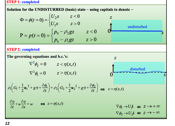
Kelvin helmholtz linear analysis: Base solution
the base solution can be seen in the image
now we have varying pressures
Kelvin helmholtz linear analysis: Boundary conditions
These are identical to our shear layer except for the pressure boundary condition which varies with density now.
So:
Pressure: ρ1(∂t∂ϕ1+2u12+gz+G1)=ρ2(∂t∂ϕ2+2u22+gz+G2) densities are now shown
Our steady state is now:ρ1(2u12+G1)=ρ2(2u22+G2)
Kinematic:-
Upper layer: ∂t∂η′+U1∂x∂η′=∂z∂ϕ1′on z=0
Lower layer: ∂t∂η′+U2∂x∂η′=∂z∂ϕ2′on z=0
Localisation:
∇ϕ2→U2iasz→−∞
∇ϕ1→U1iasz→+∞
Kelvin helmholtz linear analysis: Introducing perturbations
Still adding the same pertubations
Perturb velocity: u=U+u′(x,z,t)
Perturb pressure: p=P+p′(x,z,t)
Perturb 'interface': η=0+η′(x,t)
subbing this into our laplacian governing equations, we get:
\nabla^2 \phi_1' = 0 \quad \text{for } z > 0
\nabla^2 \phi_2' = 0 \quad \text{for } z < 0
Same governing equations as before
Changing z coordinate
Same analysis in shear flow where we ignore the small distance caused by the perturbations and take our values at z = 0
Linearised boundary equations
Our kinematic and localisation boundary conditions are exactly the same, when we’re linearising.
Kinematic
Upper layer: ∂t∂η′+U1∂x∂η′=∂z∂ϕ1′on z=0
Lower layer: ∂t∂η′+U2∂x∂η′=∂z∂ϕ2′on z=0
localisation:
∇ϕ2′→0 asz→−∞
∇ϕ1′→0asz→+∞
pressure
we can no longer ignore the hydrostatic term as before:
so original equation is:
ρ1(G1+2U12+U1∂x∂ϕ1′+2(∇ϕ1′)2+gη′+∂t∂ϕ1′)=ρ2(G2+2U22+U2∂x∂ϕ2′+2(∇ϕ2′)2+gη′+∂t∂ϕ2′)on z=η′
can still simplify with base state since z=η’ and z=0 is basically the same, so ⇒(21U12+G1)=(21U22+G2) on z=0
our grad squared term is small and can be removed, but no longer can remove hydrostatic term ρgη’
Find normal mode solutions
Plugging in our normal mode solutions into laplace’s equation:ϕ2′=ϕ^2(z)⋅eikx+st etc..
We have the exact same form (since same governing equations)
so:
ϕ1′==ϕ^1Be−kz⋅eikx+stϕ2′==ϕ^2Cekz⋅eikx+st
exactly the same using kinematic to find B and C
B=−(s+U1ik)kη^ and C=(s+U2ik)kη^
different pressure boundary condition for different relationship between B and C
ρ1[(s+ikU1)B+gη^]=ρ2[(s+ikU2)C+gη^]
Compare with (s+U1ik)B=(s+U2ik)C for same density
We get our quadratic now:
ρ1[kg−(s+U1ik)2]=ρ2[kg+(s+U2ik)2]
Result:
this result in a growth rate: (once solved with quadratic formula)
s=−ikρ1+ρ2ρ1U1+ρ2U2±[(ρ1+ρ2)2k2ρ1ρ2(U1−U2)2−gkρ1+ρ2(ρ2−ρ1)]1/2
Physical implication of kelvin helmholtz
Our poles for kelvin helmholtz lie on:
s=−ikρ1+ρ2ρ1U1+ρ2U2±[(ρ1+ρ2)2k2ρ1ρ2(U1−U2)2−gkρ1+ρ2(ρ2−ρ1)]1/2
This is unstable if the second term is real
Thus our stable criteria is if the second term is imaginary: so
\left[\frac{k^2\rho_1\rho_2(U_1-U_2)^2}{(\rho_1+\rho_2)^2}-gk\frac{(\rho_2-\rho_1)}{\rho_1+\rho_2}\right]<0
This results in a stability criteria of:
\Rightarrow \text{instability for wavenumbers } k > g \frac{(\rho_2^2 - \rho_1^2) / \rho_1 \rho_2}{(U_1 - U_2)^2}
Low wavelengths are stabilised by bouyancy
This is because it involves moving large masses of fluids, while at smaller scale the shear forces dominate.
Differences between uniform shear and kelvin helmholtz
Energy analysis of general stratification
We can form a criterion for stratification by considering work.
We are considering two particles swapping places
Change in work from bouyancy
Change in kinetic energy
This is unstable if ΔKE > work done against bouyancy
Looking at a continuous strata where our density and velocity varies continuously with height.
Work done against bouyancy:
Fbuoy={density of particleρ(z)−ρ(z+a) density of environment[ρ(z)+adzdρ+…]}gV≈−(adzdρ)gV
work done=∫a=0a=δzFbuoy⋅dr=∫0δz−(adzdρgV)da=−21(δz)2dzdρgV
change in kinetic energy:
Kinetic energy before switching: (density changes don’t affect KE, only hydrostatic)
KEbefore=21m1u2+21m2(u+δu)2where m1≈m2=ρ0V
Kinetic energy after swapping: (assuming they take mean velocity)
KEafter=21m1(2u+(u+δu))2+21m2(2u+(u+δu))2
change is thus:
ΔKE=KEbefore−KEafter=4ρ0V(δu)2
Unstable if:
\frac{\rho_0 V}{4}(\delta u)^2 > -2 \times \frac{1}{2} (\delta z)^2 \frac{d\rho}{dz} gV (two added for two particles)
If we’re taking this as a derivative by δu/δz ≈ du/dz
\frac{1}{4} > \frac{-\frac{g}{\rho_0} \frac{d\rho}{dz}}{\left( \frac{du}{dz} \right)^2} = \frac{N^2}{\left( \frac{du}{dz} \right)^2}
This dimensionless ratio is the Richardson Number ($Ri$).
Ri=(du/dz)2N2
Condition for instability: $Ri < \frac{1}{4}$
![<p>We can form a criterion for stratification by considering work.</p><ul><li><p>We are considering two particles swapping places</p></li><li><p>Change in work from bouyancy</p></li><li><p>Change in kinetic energy</p></li></ul><p><strong>This is unstable if ΔKE > work done against bouyancy</strong> </p><p></p><p>Looking at a continuous strata where our density and velocity varies continuously with height.</p><p><strong>Work done against bouyancy</strong>:</p><p>$$F_{buoy} = \{ \underbrace{\rho(z)}_{\text{density of particle}} - \underbrace{[\rho(z) + a \frac{d\rho}{dz} + \dots]}_{\rho(z+a) \text{ density of environment}} \} gV \approx -\left( a \frac{d\rho}{dz} \right) gV$$ </p><p>$$\text{work done} = \int_{a=0}^{a=\delta z} F_{buoy} \cdot d\mathbf{r} = \int_{0}^{\delta z} -\left( a \frac{d\rho}{dz} gV \right) da = -\frac{1}{2}(\delta z)^2 \frac{d\rho}{dz} gV$$ </p><p></p><p><strong>change in kinetic energy</strong>: </p><ul><li><p>Kinetic energy before switching: <strong>(density changes don’t affect KE, only hydrostatic)</strong></p><ul><li><p>$$KE_{before} = \frac{1}{2}m_1 u^2 + \frac{1}{2}m_2 (u + \delta u)^2 \quad \text{where } m_1 \approx m_2 = \rho_0 V$$ </p></li></ul></li><li><p>Kinetic energy after swapping: <strong>(assuming they take mean velocity)</strong></p><ul><li><p>$$KE_{after} = \frac{1}{2}m_1 \left( \frac{u + (u + \delta u)}{2} \right)^2 + \frac{1}{2}m_2 \left( \frac{u + (u + \delta u)}{2} \right)^2$$ </p></li></ul></li></ul><p>change is thus:</p><p>$$\Delta KE = KE_{before} - KE_{after} = \frac{\rho_0 V}{4}(\delta u)^2$$ </p><p></p><p><strong>Unstable if</strong>:</p><p>$$\frac{\rho_0 V}{4}(\delta u)^2 > -2 \times \frac{1}{2} (\delta z)^2 \frac{d\rho}{dz} gV$$ (two added for two particles)</p><p></p><p>If we’re taking this as a derivative by δu/δz ≈ du/dz</p><p>$$\frac{1}{4} > \frac{-\frac{g}{\rho_0} \frac{d\rho}{dz}}{\left( \frac{du}{dz} \right)^2} = \frac{N^2}{\left( \frac{du}{dz} \right)^2}$$ </p><p></p><p>This dimensionless ratio is the <strong>Richardson Number (</strong><span><strong>$Ri$</strong></span><strong>)</strong>.</p><p>$$Ri = \frac{N^2}{(du/dz)^2}$$</p><p><strong>Condition for instability: </strong><span><strong>$Ri < \frac{1}{4}$</strong></span></p>](https://assets.knowt.com/user-attachments/0b48936d-551b-4012-a959-96841bfe56ce.png)
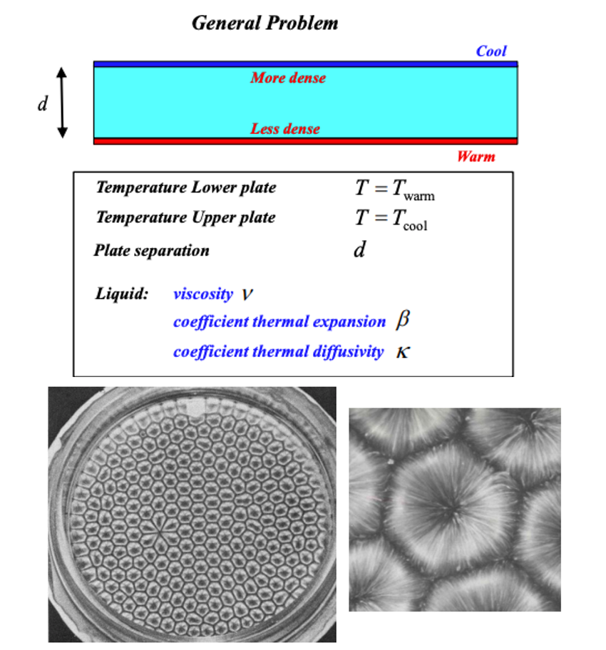
Rayleigh bernard convection overview
Here we have a similar flow structure to taylor courette, modelling the flow between two plates at different temperatures:
The steady state solution is just diffusive flow, where we have heat diffusion from one side to another
We have a convective mode solution, where bouyancy results in instability
Analogy to taylor courette
There is an exact analogy to thin gap taylor courette
In taylor courette we have the taylor number T=ν2r12(Ω1r12−Ω2r22)Ωd3≈viscosityinertia
In rayleigh bernard we have the rayleigh number: Ra = \frac{g \beta \Delta T d^3}{\kappa \nu} > Ra_{crit}
Both of these result in stability when we exceed 1708
There is a perfect physical analogy here too
In taylor courette, if we enter a rotating frame. We have an instability driven by a centrifugal force, with a fixed boundary at the two walls.
This centrifugal force is constant with r just like a constant g for a thin gap
In rayleigh bernard. We have an instability driven by bouyancy (gravity field) (temperature), with a fixed boundary at two walls
Base case both have a linear potential field (centrifugal driven, and gravity) (when small gap)
This is destabilising against viscosity
This is why we result in the same maths
Rayleigh bernard linear analysis: Governing equations and boundary equations
Governing equations:
Our governing equations are:
Navier stokes: ∂t∂u+(u⋅∇)u=−ρ1∇p+ν∇2u+g (assume viscosity constant with temperature)
continuity: DtDρ+ρ∇⋅u=0Density variations smallDtDρ=0⟹∇⋅u=0 (assume constant density for continuity)
Thermal diffusion: ∂t∂T+(u⋅∇)T=κ∇2T
Equation of state: ρ=ρ~[1−β(T−T~)]
Compared to taylor-courette
Same navier stokes and continuity to govern the fluid flow
Our thermal diffusion is lumped within navier stokes, as it is momentum diffusion that results the change in fluid energy
No equation of state, also lumped into navier stokes as a centrifugal force term.
Boundary conditions:
Temperature BC
T=Tcool on z=d for all t.
T=Twarm on z=0 for all t.
This is analogous to our no slip condition in taylor courette, as both of these boundary conditions define a fluid energy within our system
Velocity BC
No flow through boundaries: Vertical velocity w=0 at the walls.
No slip: Horizontal velocities u=v=0 at the walls.
Same as taylor-courette
We can see how for the boundary conditions too, taylor courette sort of lumps terms together
Rayleigh bernard linear analysis: Base flow solution
This base flow involves no motion, so our base flow is purely a heat diffusion equation.
Solving steady temperature diffusion equation:
∂t∂T+(U⋅∇)T=κ∇2T
No transport or unsteady term, so just a laplacian solution:
0+0=κdz2d2T0(z)
Plugging in our boundary conditions this has the following solution:
T0(z)=Twarm−dz(Twarm−Tcool)
With analogous pressure and density solutions:
Density: ρ0(z)=ρ~[1−β(T0(z)−T~)]
Pressure: dzdP0=−ρ0(z)g
Analogy to taylor couette
This is exactly analogous to the thin gap taylor couette solution
In a thin gap we get a linear increase in azimuthal velocity
In a rotating frame the flow is also steady
But like here, we have an decrease in flow energy from one plate to the other, but driven by momentum diffusion rather than thermal diffusion
Our centrifugal potential energy decreases
Compared to our gravitational potential energy
Rayleigh bernard linear analysis: Introducing perturbations and finding PDE
Perturbations:
We are introducing the following perturbations:
Velocity: u=0+u′[cite: 173]
Temperature T=T0(z)+T′[cite: 173]
Density: ρ=ρ0(z)+ρ′[cite: 174]
pressure p=P0(z)+p′[cite: 174]
Plugging into governing equations
Remember our governing equations are:
Navier stokes: ∂t∂u+(u⋅∇)u=−ρ1∇p+ν∇2u+g (assume viscosity constant with temperature)
continuity: DtDρ+ρ∇⋅u=0Density variations smallDtDρ=0⟹∇⋅u=0 (assume constant density for continuity)
Thermal diffusion: ∂t∂T+(u⋅∇)T=κ∇2T
Equation of state: ρ=ρ~[1−β(T−T~)]
Plugging into navier stokes
When plugging into navier stokes we get:
(ρ0+ρ′)[∂t∂u′+(u′⋅∇)u′]=−∇(P0+p′)+(ρ0+ρ′)ν∇2u′+(ρ0+ρ′)g
Now ignoring products of small temrs and introducing a hydrostatic balance dzdP0=−ρ0g
ρ0∂t∂u′=−∇p′+ρ0ν∇2u′+ρ′g
Because density changes are small, we are rewriting it in terms of a constant reference density
ρ~∂t∂u′=−∇p′+ρ~ν∇2u′+ρ′g[cite: 194]
Other governing equations
Continuity: we get ∇⋅u′=0
Thermal diffusion: we get: ∂t∂T′+w′(dzdT0)=κ∇2T′
Equation of state: ρ′=−βρ~T′
Combining linearised governing equations:
Our goal is an expression for vertical velocity This is because convection gives vertical velocity
Eliminate pressure in NS
We can take the curl to eliminate pressure (as it is a potential field)
(∂t∂−ν∇2)∇×u′=−β(∇T′)×g
If we take the curl again, we can simplify further with the identities
∇×∇×u′=∇(∇⋅u′)−∇2u′ and ∇⋅u′=0, leaving just a laplacian term
⇒−(∂t∂−ν∇2)∇2u′=−∇×(β(∇T′)×g) which simplifies with more vector identities to:
∇×(F×G)=(G⋅∇)F−(F⋅∇)G+F(∇⋅G)−G(∇⋅F) so:
∇×[β(∇T′)×g]=(g⋅∇)β(∇T′)−=0 as ∇g=0(β(∇T′)⋅∇)g+=0 as ∇⋅g=0β(∇T′)(∇⋅g)−g(∇⋅β(∇T′))
(∂t∂−ν∇2)∇2u′=β[(g⋅∇)∇T′−g∇2T′]
looking at vertical component
Using the fact gravity only acts in vertical direction g = (0,0,-g)
(∂t∂−ν∇2)∇2w′=βg(∂x2∂2+∂y2∂2)T′
eliminate temperature perturbation (so we just have our equation in w’)
We will use the energy equation to do this, rewriting our energy equation we get:
∂t∂T′+w′(dzdT0)=κ∇2T′ rearranging we get:
(∂t∂−κ∇2)T′=−w′dzdT0[cite:267]
PDE solution
Subbing this into the vertical component equation we get:
(∂t∂−κ∇2)(∂t∂−ν∇2)∇2w′=−βg(∂x2∂2+∂y2∂2)w′dzdT0[cite:270]
Rayleigh bernard linear analysis: Solving PDE
Forming ODE and comparing to taylor-courette
Our PDE is now: (∂t∂−κ∇2)(∂t∂−ν∇2)∇2w′=−βg′dzdT0(∂x2∂2+∂y2∂2)w′
compare with taylor-courette:
(∂t∂−ν∇~2)∇~2ur′=(r2Uθ)∂z2∂2uθ′
(∂t∂−ν∇~2)uθ′+(2A)ur′=0 if we sub in for uθ in the derivative
(∂t∂−ν∇2)(∂t∂−ν∇2)∇2ur′=−(2A)r2Uθ[∂z2∂2]ur′
Exactly in the same form: The Two Brakes(∂t∂−Diff1)(∂t∂−Diff2)Stabilizing Curvature∇2Ψ′=Coupling−CEnergy Gradient(dηdΦ0)Symmetry-Breaking Laplacian∇⊥2Ψ′
we have different geometry though, since taylor-courette our cells must be stacked vertically, while in rayleigh bernard they can spread out in a plane
Applying modal solutions
We assume a solution of the form:
w′=w^(z)f(x,y)est
w^(z): The unknown vertical structure of the roll.
f(x,y): The horizontal pattern; we assume there is no preferred horizontal direction.
est: Introduces the growth rate (s) to determine if the perturbation grows (s > 0) or decays.
This gives us the ODE
[ν(dz2d2−a2)−s][κ(dz2d2−a2)−s](dz2d2−a2)w^=(βgdzdT0a2)w^
Workings for the Substitution:
Temporal derivative: ∂t∂w′=sf(x,y)estw^
Spatial Laplacian: ∇2w′=[(∂x2∂2f+∂y2∂2f)est+festdz2d2]w^=(dz2d2−a2)festw^
Applying boundary conditions
We need 6 boundary conditions for w’
No penetration boundary condition: w′=0⟹w^=0 at z=(0,d)
no slip boundary condition dzdw^=0on z=(0,d) (from no slip and continuity)
energy anchor boundary condition T′=0 on z=(0,d)
Applying this simplified navier stokes (∂t∂−ν∇2)∇2w′=βg(∂x2∂2+∂y2∂2)T′ so we get this in terms of w’
We get: (∂t∂−ν∇2)∇2w′z=0,d=0 which when differentiated and with our modal solution gets us
dz4d4w^−(2a2+s/ν)dz2d2w^z=0,d=0
Again analogous to taylor-courette, we have the same two no penetration and no slip boundary conditions
This condition: dr4d4u^r−(2k2+νs)dr2d2u^r=0on r=(r1,r2) is equivalent to a uθ′=0 condition in uᵣ This is an energy anchor condition
Solution:
we get an identical solution to taylor courette as shown in picture.
if we solve with the simplified boundary condition set so:
No-Slip: w^=0 ⟶ Stress-Free: w^=0 (no change)
No-Slip: dzdw^=0 ⟶ Stress-Free: dz2d2w^=0 (from no slip to no shear stress)
No-Slip: dz4d4w^−(2a2+s/ν)dz2d2w^=0 ⟶ Stress-Free: dz4d4w^=0 (follows from previous assumptions)
This enables our sinusoidal solution:
w^=sin(Nπdz)
stability criteria
With our simplified boundary conditions, we’re looking when the wave number is 1
We find a definition for the rayleigh number in terms of our wavenumber by plugging the sin solution into the ODE
Ra=a2d4[d2N2π2+a2]3
Critical rayleigh number is the minimum value of this when N = 1, equals 658
Our real value is 1708 like with taylor courette
![<h4 id="be76c8b1-337c-4597-bccc-dd51f55e70f2" data-toc-id="be76c8b1-337c-4597-bccc-dd51f55e70f2" collapsed="false" seolevelmigrated="true">Forming ODE and comparing to taylor-courette</h4><p>Our PDE is now: $$\left(\frac{\partial}{\partial t}-\kappa\nabla^2\right)\left(\frac{\partial}{\partial t}-\nu\nabla^2\right)\nabla^2w^{\prime}=-\beta g^{\prime}\frac{dT_0}{dz}\left(\frac{\partial^2}{\partial x^2}+\frac{\partial^2}{\partial y^2}\right)w^{\prime}$$</p><ul><li><p><strong>compare with taylor-courette</strong>:</p><ul><li><p>$$\left( \frac{\partial}{\partial t} - \nu \tilde{\nabla}^2 \right) \tilde{\nabla}^2 u_r' = \left( \frac{2U_\theta}{r} \right) \frac{\partial^2 u_\theta'}{\partial z^2}$$</p></li><li><p>$$\left( \frac{\partial}{\partial t} - \nu \tilde{\nabla}^2 \right) u_\theta' + (2A) u_r' = 0$$ if we sub in for uθ in the derivative</p></li><li><p>$$\left(\frac{\partial}{\partial t}-\nu\nabla^2\right)\left(\frac{\partial}{\partial t}-\nu\nabla^2\right)\nabla^2u_{r}^{\prime}=-(2A)\frac{2U_\theta}{r}\left[\frac{\partial^2}{\partial z^2}\right]u_{r}^{\prime}$$</p></li></ul></li><li><p>Exactly in the same form: $$\underbrace{\left(\frac{\partial}{\partial t}-\text{Diff}_1\right)\left(\frac{\partial}{\partial t}-\text{Diff}_2\right)}_{\text{The Two Brakes}}\underbrace{\nabla^2\Psi^{\prime}}_{\text{Stabilizing Curvature}}=\underbrace{-\mathcal{C}}_{\text{Coupling}}\underbrace{\left(\frac{d\Phi_0}{d\eta}\right)}_{\text{Energy Gradient}}\underbrace{\nabla_{\perp}^2\Psi^{\prime}}_{\text{Symmetry-Breaking Laplacian}}\text{ }$$</p></li><li><p>we have different geometry though, since taylor-courette our cells must be stacked vertically, while in rayleigh bernard they can spread out in a plane</p></li></ul><p></p><p><strong>Applying modal solutions</strong></p><p><span style="line-height: 1.15;">We assume a solution of the form</span>:</p><p>$$w' = \hat{w}(z) f(x,y) e^{st}$$</p><ul><li><p><span style="line-height: 1.15;"><strong>$$\hat{w}(z)$$</strong>: The unknown vertical structure of the roll.</span></p></li><li><p><span style="line-height: 1.15;"><strong>$$f(x,y)$$</strong>: The horizontal pattern; we assume there is no preferred horizontal direction.</span></p></li><li><p><span style="line-height: 1.15;"><strong>$$e^{st}$$</strong>: Introduces the growth rate ($$s$$) to determine if the perturbation grows ($$s > 0$$) or decays.</span></p></li></ul><p></p><p>This gives us the ODE</p><p>$$\left[ \nu \left( \frac{d^2}{dz^2} - a^2 \right) - s \right] \left[ \kappa \left( \frac{d^2}{dz^2} - a^2 \right) - s \right] \left( \frac{d^2}{dz^2} - a^2 \right) \hat{w} = \left( \beta g \frac{dT_0}{dz} a^2 \right) \hat{w}$$</p><p><span style="line-height: 1.15;">Workings for the Substitution</span>:</p><ul><li><p>Temporal derivative: $$\frac{\partial}{\partial t} w' = s f(x,y) e^{st} \hat{w}$$</p></li><li><p>Spatial Laplacian: $$\nabla^2 w' = \left[ \left( \frac{\partial^2 f}{\partial x^2} + \frac{\partial^2 f}{\partial y^2} \right) e^{st} + f e^{st} \frac{d^2}{dz^2} \right] \hat{w} = \left( \frac{d^2}{dz^2} - a^2 \right) f e^{st} \hat{w}$$</p></li></ul><p></p><h4 id="9dffad2a-3cb1-445d-b889-e87c9d5b07db" data-toc-id="9dffad2a-3cb1-445d-b889-e87c9d5b07db" collapsed="false" seolevelmigrated="true">Applying boundary conditions</h4><p>We need 6 boundary conditions for w’</p><ul><li><p><strong>No penetration boundary condition</strong>: $$w^{\prime}=0\implies\hat{w}=0\space at \space z=(0,d)$$</p></li><li><p><strong>no slip boundary condition</strong> $$\frac{d\hat{w}}{dz} = 0 \quad \text{on } z = (0, d)$$ (from no slip and continuity)</p></li><li><p><strong>energy anchor boundary condition</strong> $$T' = 0$$ on $$z = (0, d)$$</p><ul><li><p>Applying this simplified navier stokes $$\left( \frac{\partial}{\partial t} - \nu \nabla^2 \right) \nabla^2 w' = \beta g \left( \frac{\partial^2}{\partial x^2} + \frac{\partial^2}{\partial y^2} \right) T'$$ so we get this in terms of w’</p></li><li><p>We get: $$\left.\left(\frac{\partial}{\partial t}-\nu\nabla^2\right)\nabla^2w^{\prime}\right|_{z=0,d}=0$$ which when differentiated and with our modal solution gets us</p></li><li><p>$$\left.\frac{d^4 \hat{w}}{dz^4}-\left(2a^2+s/\nu\right)\frac{d^2 \hat{w}}{dz^2}\right|_{z=0,d}=0$$</p><p></p></li></ul></li></ul><p></p><p>Again analogous to taylor-courette, we have the same two no penetration and no slip boundary conditions</p><ul><li><p>This condition: $$\frac{d^4 \hat{u}_r}{dr^4} - \left( 2k^2 + \frac{s}{\nu} \right) \frac{d^2 \hat{u}_r}{dr^2} = 0 \quad \text{on } r = (r_1, r_2) \text{}$$ is equivalent to a $$u_\theta' = 0$$ condition in uᵣ <strong>This is an energy anchor condition</strong></p></li></ul><p></p><h4 id="3c8542b9-7fbe-4add-8447-80030850c02b" data-toc-id="3c8542b9-7fbe-4add-8447-80030850c02b" collapsed="false" seolevelmigrated="true">Solution:</h4><p>we get an identical solution to taylor courette as shown in picture.</p><p>if we solve with the simplified boundary condition set so:</p><ul><li><p><strong>No-Slip:</strong> <span>$$\hat{w} = 0$$</span> <span>$$\quad \longrightarrow \quad$$</span> <strong>Stress-Free:</strong> <span>$$\hat{w} = 0$$ (no change)</span></p></li><li><p><strong>No-Slip:</strong> <span>$$\frac{d\hat{w}}{dz} = 0$$</span> <span>$$\quad \longrightarrow \quad$$</span> <strong>Stress-Free:</strong> <span>$$\frac{d^2\hat{w}}{dz^2} = 0$$ (from no slip to no shear stress)</span></p></li><li><p><strong>No-Slip:</strong> <span>$$\frac{d^4 \hat{w}}{dz^4} - (2a^2 + s/\nu)\frac{d^2 \hat{w}}{dz^2} = 0$$</span> <span>$$\quad \longrightarrow \quad$$</span> <strong>Stress-Free:</strong> <span>$$\frac{d^4 \hat{w}}{dz^4} = 0$$ (follows from previous assumptions)</span><br></p></li></ul><p>This enables our sinusoidal solution:</p><p>$$\hat{w}=\sin\left(N\pi\frac{z}{d}\right)$$ </p><p></p><h3 id="bdc47abf-61c2-4c42-b027-adbd602a2d81" data-toc-id="bdc47abf-61c2-4c42-b027-adbd602a2d81" collapsed="false" seolevelmigrated="true">stability criteria</h3><p>With our simplified boundary conditions, we’re looking when the wave number is 1</p><p>We find a definition for the rayleigh number in terms of our wavenumber by plugging the sin solution into the ODE</p><p>$$Ra = \frac{d^4}{a^2} \left[ \frac{N^2\pi^2}{d^2} + a^2 \right]^3$$ </p><ul><li><p>Critical rayleigh number is the minimum value of this when N = 1, equals 658</p></li></ul><p></p><p>Our real value is 1708 like with taylor courette</p><p></p><p></p><p></p>](https://assets.knowt.com/user-attachments/5f279d3b-b850-4508-974a-5328bb3b8f37.png)
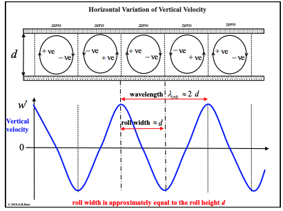
Flow structure of rayleigh-bernard
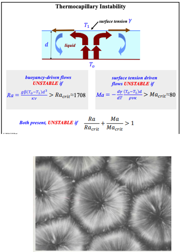
Bernard Marangoni
This looks similar to rayleigh bernard, but the driving force is NOT a density gradient due to temperature but rather a surface tension gradient due to temperature.
This is defined by a different Maragoni number
This is unstable ifMa=−dTdγρνκ(T0−T1)d > 80
Often both effects are combined, described by if \frac{Ra}{Ra_{crit}} + \frac{Ma}{Ma_{crit}} > 1
Rayleigh dominates for thicker layers
Role of symmetry breaking in instability
Instability can often been seen in the perspective of breaking symmetries:
The 4 Core Examples of Symmetry Breaking
Type of Symmetry | The "Perfect" (Symmetric) State | The Broken (Instability) State | Example |
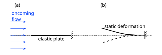
Reflection | A flat plate aligned perfectly with a steady flow. | The plate spontaneously bends to one side. | A cantilevered postcard in the wind. |
Time-Translation | A steady input (like blowing air at a constant rate). | The output becomes oscillatory (vibration). | Blowing a raspberry or vocal cords vibrating. |
Spatial Translation | An infinitely long, uniform thread of liquid. | The thread pinches off into individual droplets. | Rayleigh-Plateau instability (dripping tap). |
Axisymmetry | Wine coating a glass in a perfect, smooth circle. | The wine falls in distinct, repeating "tears" or legs. | Marangoni effect (tears of wine). |
Role of positive feedback in breaking symmetry
Symmetries are often broken through positive feedback loops.
Example of aeroelastic divergence:
If we consider a wing with a centre of lift infront of the torsional center
Doing a torque balance: T=Fluid Torque (Destabilizing)21CLρU2cwdsinθcosθ−Spring Torque (Restoring)κθ
We can see we get an increasing torque, if:
\frac{C_L \rho U^2 c w d}{2\kappa} > \frac{\theta}{\sin \theta \cos \theta}
This was a big issue with early flight.
Formalising analysis of lienar stability theory
Comparing with the picture there are 8 steps to linear analysis.
1. State and state variables
We first need to find the quantities we are using the define the system, these are our state variables.
For the aeroelastic plate example, the system state is only defined by θ(t)
2. Governing dynamics
We then need to work out the equations that link our state variables together and define our system.
dtdx=F(x;p) (our equation for how our variable changes over time)
This depends on our state variables (x) like position, and system parameters (p) like density, freestream velocity etc.
Enslaved variables:
Many variables respond so quickly that they are “enslaved” to others
For instance our lift force is enslaved to θ, since we assume the flow field responds fast enough to reach a steady state
As such we are describing the system with just θ
symmetries and approximations
Many systems are invariant in our state variables, and have symmetries
Ie our plate situation is symmetric about θ, and also time invariant (where a shift in time doesn’t change F)
3. Steady state
We first want to find a steady state solution, this should obey the symmetry which is being broken by the instability ie:
Time-Translation Symmetry: We look for a state where $$\theta</span>orvelocityisconstant.Itlooksthesamewhetheryoulooknowortenminutesfromnow.</p></li><li><p><strong>SpatialTranslationSymmetry:</strong>Inaliquidthread(Rayleigh−Plateau),thesteadystateisaperfectcylinder.Everypointalongtheaxisisidentical.</p></li><li><p><strong>ReflectionSymmetry:</strong>Foryourhingedplate,thesteadystateis<span>\theta = 0</span>.Thisistheonlystatethatisidenticaltoitsmirrorimage.</p></li></ul><p></p><p><strong>Floquetanalysis</strong></p><p>Somesystemsdon’thaveasteadystateintime,suchaperiodicsystemslikeaswing</p><ul><li><p>Wethenconsiderifthereisgrowthafteraperiod.</p></li></ul><p></p><h4id="8f04a236−725d−4f2c−a268−6362b7a323e9"data−toc−id="8f04a236−725d−4f2c−a268−6362b7a323e9"collapsed="false"seolevelmigrated="true">4.Introducingaperturbation</h4><p>Wearenowintroducingaperturbationontooursteadystate.Ienudgingourstate,.</p><p>\mathbf{x} = \mathbf{x}_0 + \mathbf{x}' \quad (1.7)</p><p>Asoursteadystateisbydefinitionnotchanging,wecananalysethesystembyhowthisperturbationvaries</p><p>\frac{d\mathbf{x}'}{dt} = \mathcal{F}(\mathbf{x}_0 + \mathbf{x}'; p) \quad (1.8)</p><p></p><h4id="7e237f6a−0706−450a−b858−7c821cb310b4"data−toc−id="7e237f6a−0706−450a−b858−7c821cb310b4"collapsed="false"seolevelmigrated="true">5.Linearisation</h4><p>Byconsideringonlyverysmallperturbationsweareabletolineariseourgoverningequations</p><p>\mathcal{F}(x_0 + x'; p) = \underbrace{\mathcal{F}(x_0; p)}_{= 0} + \underbrace{\frac{\delta \mathcal{F}}{\delta x}(x_0; p) x'}_{\text{Linear Term}} + \text{Higher Order Terms (H.O.T.)}</p><ul><li><p>Slightcaveatofourgoverningequationsmustbesmooth(differentiable)butthisistrueformostsystems</p></li></ul><p></p><h4id="d26c3f97−efb9−43b3−b718−22c704baefce"data−toc−id="d26c3f97−efb9−43b3−b718−22c704baefce"collapsed="false"seolevelmigrated="true">6.Nondimensionalising</h4><p>Thisisanoptionalstep,butoftenhelpsunderstandthesystem</p><ul><li><p>Suchasnormalisingwithalengthscale,orfindingatimescale</p></li><li><p>Helpsfindnondimensionalparametersthatdefinethesystemlike<strong>reynoldsnumbers,rayleighnumber</strong></p></li></ul><p></p><h4id="69aa0805−8626−469e−bf73−889d73f9e03c"data−toc−id="69aa0805−8626−469e−bf73−889d73f9e03c"collapsed="false"seolevelmigrated="true">7.Normalmodesandexponentialgrowth</h4><ul><li><p>Thisisbecausewehavelinearisedoursystemsosuperpositionapplies</p></li><li><p>Becauseofthetimeinvarianceanexponentialsolutionmustbeapply,</p></li><li><p>Assuchwehaveaneigenvalueproblem,s\hat{\mathbf{x}} = \mathcal{L}\hat{\mathbf{x}}</p></li></ul><p></p><h4id="c052cc37−4153−4335−bbdf−d85c15351647"data−toc−id="c052cc37−4153−4335−bbdf−d85c15351647"collapsed="false"seolevelmigrated="true">8.Conditionsforinstability</h4><ul><li><p>Thisisbasicallyifwehaveanypoless,wherehavepositiverealvalues</p></li></ul><tablestyle="min−width:75px;"><colgroup><colstyle="min−width:25px;"><colstyle="min−width:25px;"><colstyle="min−width:25px;"></colgroup><tbody><tr><tdcolspan="1"rowspan="1"style="animation:autoease0s1normalnonerunningnone;appearance:none;background:none0\Re(s_1) < 0</span></p></td></tr><tr><tdcolspan="1"rowspan="1"style="animation:autoease0s1normalnonerunningnone;appearance:none;background:none0\Re(s_1) = 0</span></p></td></tr><tr><tdcolspan="1"rowspan="1"style="animation:autoease0s1normalnonerunningnone;appearance:none;background:none0\Re(s_1) > 0$$
Example of a structural system : Mass spring damper
Modelling equations
This is described by a second order differential equation
mx¨+bx˙+kx=f (where f is a driving function). This is already linear
We can also take an energy perspective, multiplying the force by the velocity to get the work.
so for this is it dtd[21m(dtdx)2+21kx2]=−b(dtdx)2+fdtdx
We have our conservative KE and PE terms on LHS. Damper and energy addition via external work too.
Matrix form
For two degrees of freedom (with no damping) say if we have a system in the form: (for pitch and heave)
mh¨+kh+kxssinθ=L
Iθ¨+kxshcosθ+κθ=Lxacosθ
we can rewrite this coupled equation in terms of a mass and stiffness matrix. where the state vector x=[h,θ]T
Mx¨+Kx=0 where M=(m0amp;0amp;I) and K=(kkxsamp;kxsamp;κ)
energy formulation
Our kinetic and potential energy of this system can be written as the below, where we have energy conservation.
dtd[21x˙TMx˙+21xTKx]=0
Eigenvector equation:
We want to solve the for eigenvalues which are our natural frequencies. As x=¨−ω2x
This is the determinant of (K−ω2M)x^=0
We would then plug in our eigenvalues to find the eigenvectors which are our mode shapes
Remember to note symmetric systems have orthogonal eigenvectors
Non dimensionalisation:
We can non dimensionlise our variables.
t=t~km,h′=Rgh~,θ′=θ~,δ=Rg2xs,andωa2=kRg2κ
Basically dividing by our natural frequency of heave, radius of gyration, our ratio between heave to CoM and radius of gyration and our ratio of torsional to translational stiffness
Very large systems and rayleigh’s quotient
We can represent increasingly large systems with just a larger state vector.
Mdt2d2x′+Kx′=0
We can represent any response as a linear combination of our eigenvector modes, as a modal summation
i=1∑n(a¨i+ωi2ai)Mx^i=f
As these modes are orthogonal, if we dot this with an eigenvector x^j, it only leaves the i = j term.
Hence: (a¨j+ωj2aj)(x^jTMx^j)=x^jTf
and: a¨j+ωj2aj=x^jTMx^jx^jTf
![<h4 id="ab5ddd47-887f-4462-bcb9-31f7df9fc654" data-toc-id="ab5ddd47-887f-4462-bcb9-31f7df9fc654" collapsed="false" seolevelmigrated="true">Modelling equations</h4><p>This is described by a second order differential equation</p><p><span style="line-height: 1.15;">$$m\ddot{x} + b\dot{x} + kx = f$$ (where f is a driving function). <strong>This is already linear</strong></span></p><p><strong>We can also take an energy perspective,</strong> multiplying the force by the velocity to get the work.</p><ul><li><p>so for this is it $$\frac{d}{dt}\left[\frac{1}{2}m\left(\frac{dx}{dt}\right)^2+\frac{1}{2}kx^2\right]=-b\left(\frac{dx}{dt}\right)^2+f\frac{dx}{dt}$$</p></li><li><p>We have our conservative KE and PE terms on LHS. Damper and energy addition via external work too.</p></li></ul><p></p><p></p><p></p><h3 id="122b0113-7839-4d28-8425-038328f5e641" data-toc-id="122b0113-7839-4d28-8425-038328f5e641" collapsed="false" seolevelmigrated="true">Matrix form</h3><p>For two degrees of freedom <strong>(with no damping)</strong> say if we have a system in the form: (for pitch and heave)</p><ul><li><p>$$m\ddot{h}+kh+kx_{s}\sin\theta=L$$</p></li></ul><ul><li><p>$$I\ddot{\theta}+kx_{s}h\cos\theta+\kappa\theta=Lx_{a}\cos\theta$$</p></li></ul><p>we can rewrite this coupled equation in terms of a mass and stiffness matrix. where the state vector $$\mathbf{x} = [h, \theta]^T$$ </p><p>$$\mathbf{M}\ddot{\mathbf{x}} + \mathbf{Kx} = 0$$ where $$\mathbf{M} = \begin{pmatrix} m & 0 \\ 0 & I \end{pmatrix}$$ and $$\mathbf{K} = \begin{pmatrix} k & kx_s \\ kx_s & \kappa \end{pmatrix}$$</p><p><strong> energy formulation</strong></p><p>Our kinetic and potential energy of this system can be written as the below, where we have energy conservation.</p><p>$$\frac{d}{dt}\left[\frac{1}{2}\dot{\mathbf{x}}^{T}\mathbf{M}\dot{\mathbf{x}}+\frac{1}{2}\mathbf{x}^{T}\mathbf{Kx}\right]=0$$ </p><p></p><p><strong>Eigenvector equation:</strong></p><p>We want to solve the for eigenvalues which are our natural frequencies. As $$x\ddot = -\omega² x$$ </p><ul><li><p>This is the determinant of $$(K - \omega^2 M)\hat{x} = 0$$</p></li><li><p>We would then plug in our eigenvalues to find the eigenvectors which are our <strong>mode shapes</strong></p></li><li><p>Remember to note symmetric systems have orthogonal eigenvectors</p></li></ul><h3 id="00a8342a-e88f-4f33-acc0-1cee22a41b2c" data-toc-id="00a8342a-e88f-4f33-acc0-1cee22a41b2c" collapsed="false" seolevelmigrated="true">Non dimensionalisation:</h3><p>We can non dimensionlise our variables. </p><p>$$t=\tilde{t}\sqrt{\frac{m}{k}},\quad h^{\prime}=R_{g}\tilde{h},\quad\theta^{\prime}=\tilde{\theta},\quad\delta=\frac{2x_s}{R_g},\quad\text{and}\quad\omega_{a}^2=\frac{\kappa}{kR_g^2}$$ </p><p>Basically dividing by our natural frequency of heave, radius of gyration, our ratio between heave to CoM and radius of gyration and our ratio of torsional to translational stiffness</p><p></p><h3 id="10f46314-1bf6-41f6-9519-33da58c58a97" data-toc-id="10f46314-1bf6-41f6-9519-33da58c58a97" collapsed="false" seolevelmigrated="true">Very large systems and rayleigh’s quotient</h3><p>We can represent increasingly large systems with just a larger state vector. </p><p>$$\mathbf{M}\frac{d^{2}\mathbf{x}'}{dt^{2}}+\mathbf{Kx}^{\prime}=0$$ </p><p>We can represent any response as a linear combination of our eigenvector modes, as a modal summation</p><p>$$\sum_{i=1}^{n}(\ddot{a}_{i}+\omega_{i}^2a_{i})\mathbf{M}\hat{\mathbf{x}}_{i}=\mathbf{f}$$ </p><p>As these modes are orthogonal, if we dot this with an eigenvector <span>$$\hat{\mathbf{x}}_j$$, it only leaves the i = j term.</span></p><p><span>Hence: </span>$$(\ddot{a}_j + \omega_j^2 a_j) (\hat{\mathbf{x}}_j^T \mathbf{M} \hat{\mathbf{x}}_j) = \hat{\mathbf{x}}_j^T \mathbf{f}$$ </p><p>and: $$\ddot{a}_{j}+\omega_{j}^2a_{j}=\frac{\hat{\mathbf{x}}_j^T \mathbf{f}}{\hat{\mathbf{x}}_j^T \mathbf{M} \hat{\mathbf{x}}_j}$$ </p><p></p><p></p>](https://assets.knowt.com/user-attachments/3e275350-c41b-4ef7-becb-3d5d8189d123.png)
Example of a structural system : Continuous string system
This is now a continuous system, with a stretched string or membrane.
Derivation of response
if we consider a free small element, our vertical force balance
(μΔx)∂t2∂2y=T[(∂x∂y)x+Δx−(∂x∂y)x]+fΔx plugging into f = ma, we get
μ∂t2∂2y=T[Δx(∂x∂y)x+Δx−(∂x∂y)x]+f this is basically the definition of a derivative, as Δx → 0
μ∂t2∂2y=T∂x2∂2y+f
Result
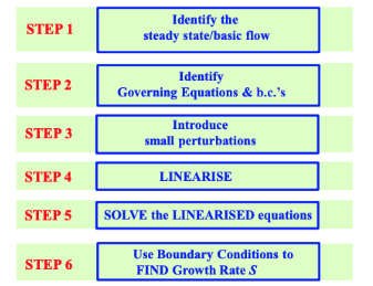
This is a PDE with a separable MODAL solution y′(x,t)=∑n=1∞an(t)y^n(x~)
Our modes will take a harmonic solution:
y^(x~)=Asin(ωx~)+Bcos(ωx~)
For this stretched string example, plugging in our boundary conditions we get y^n(x~)=sin(nπx~)
Frequency response function
we are then calculating our frequency response function.
n=1∑∞(a¨n+ωn2an)y^n(x~)=f~(x~,t~)
Now taking the integral dot product with respect to modes
∫01y^m(x~)[n=1∑∞(a¨n+ωn2an)y^n(x~)]dx~=∫01y^m(x~)f~(x~,t~)dx~
From our orthogonality condition, only the modes where n=m are non zero
a¨m+ωm2am=∫01y^m(x~)2dx~∫01y^m(x~)f~(x~,t~)dx~
This probably makes more sense in a transfer function notation, where we will consider only our modal shapes.
am(ωm2−ω2)=∫01y^m(x~)2dx~∫01y^m(x~)f~(x~,t~)dx~
now combining our mass normalisation in the denominator with our modal dot product above, we recover the 3C6 equation
H=∑ωn2−ω2uj(n)uk(n)
![<p>This is now a continuous system, with a stretched string or membrane.</p><h3 id="f6eca7eb-44e4-4b1e-9359-a969d4d5ae93" data-toc-id="f6eca7eb-44e4-4b1e-9359-a969d4d5ae93" collapsed="false" seolevelmigrated="true">Derivation of response</h3><p>if we consider a free small element, our vertical force balance</p><ul><li><p>$$(\mu \Delta x) \frac{\partial^2 y}{\partial t^2} = T \left[ \left( \frac{\partial y}{\partial x} \right)_{x+\Delta x} - \left( \frac{\partial y}{\partial x} \right)_x \right] + f \Delta x$$ plugging into f = ma, we get </p></li><li><p>$$\mu \frac{\partial^2 y}{\partial t^2} = T \left[ \frac{\left( \frac{\partial y}{\partial x} \right)_{x+\Delta x} - \left( \frac{\partial y}{\partial x} \right)_x}{\Delta x} \right] + f$$ this is basically the definition of a derivative, as Δx → 0</p></li><li><p>$$\mu\frac{\partial^2 y}{\partial t^2}=T\frac{\partial^2 y}{\partial x^2}+f$$ </p></li></ul><p></p><h3 id="09f8fcb3-806f-4ae6-8f15-888cfd665625" data-toc-id="09f8fcb3-806f-4ae6-8f15-888cfd665625" collapsed="false" seolevelmigrated="true">Result</h3><p>This is a PDE with a separable MODAL solution $$y^{\prime}(x,t)=\sum_{n=1}^{\infty}a_{n}(t)\hat{y}_{n}(\tilde{x})$$ </p><p>Our modes will take a harmonic solution:</p><p>$$\hat{y}(\tilde{x}) = A \sin(\omega \tilde{x}) + B \cos(\omega \tilde{x}) \text{}$$ </p><ul><li><p>For this stretched string example, plugging in our boundary conditions we get $$\hat{y}_{n}(\tilde{x})=\sin(n\pi\tilde{x})$$ </p></li></ul><p></p><h4 id="c2951b0e-2e5c-40e6-a7c1-511714f710fa" data-toc-id="c2951b0e-2e5c-40e6-a7c1-511714f710fa" collapsed="false" seolevelmigrated="true">Frequency response function</h4><p>we are then calculating our frequency response function.</p><p>$$\sum_{n=1}^{\infty}(\ddot{a}_{n}+\omega_{n}^2a_{n})\hat{y}_{n}(\tilde{x})=\tilde{f}(\tilde{x},\tilde{t})$$ </p><p>Now taking the integral dot product with respect to modes</p><p>$$\int_0^1\hat{y}_{m}(\tilde{x})\left[\sum_{n=1}^{\infty}(\ddot{a}_{n}+\omega_{n}^2a_{n})\hat{y}_{n}(\tilde{x})\right]d\tilde{x}=\int_0^1\hat{y}_{m}(\tilde{x})\tilde{f}(\tilde{x},\tilde{t})d\tilde{x}$$ </p><p>From our orthogonality condition, only the modes where n=m are non zero</p><p>$$\ddot{a}_{m}+\omega_{m}^2a_{m}=\frac{\int_{0}^{1} \hat{y}_m(\tilde{x}) \tilde{f}(\tilde{x}, \tilde{t}) d\tilde{x}}{\int_{0}^{1} \hat{y}_m(\tilde{x})^2 d\tilde{x}}$$ </p><p></p><p>This probably makes more sense in a transfer function notation, where we will consider only our modal shapes.</p><p>$$a_{m}\left(\omega_{m}^2-\omega^2\right)_{}=\frac{\int_{0}^{1} \hat{y}_m(\tilde{x}) \tilde{f}(\tilde{x}, \tilde{t}) d\tilde{x}}{\int_{0}^{1} \hat{y}_m(\tilde{x})^2 d\tilde{x}}$$ </p><p>now combining our mass normalisation in the denominator with our modal dot product above, we recover the 3C6 equation</p><p><span>$$H = \sum \frac{u_j^{(n)} u_k^{(n)}}{\omega_n^2 - \omega^2}$$</span></p><p></p>](https://assets.knowt.com/user-attachments/25dd67c4-27be-41f9-8f5e-05e215f6066c.png)
Example of a structural system : Euler beam
This is a 4th order continuous system,
we will first derive it for the case with no tension
Derivation of response
Again if we consider a small element, this is basically a vertical force balance but with shear forces
From classical beam theory our shear force is V=∂x∂M=B∂x3∂3y( where B=EI)
Looking at a small element on both sides, again we’re looking at the difference in shear over Δx
This results in our derivative term:
μ∂t2∂2y+B∂x4∂4y=f
Considering the free response assuming a separable modal and harmonic solution y^=exp(ωt)exp(kx)
μ∂t2∂2y+B∂x4∂4y=0
Bk4y^+μω2y^=0
now defining k as wave number of our modes, given we need an exponential modal solution
ω=k2μB=k2μEI
Our full equation if we include tension as well, is:
μ∂t2∂2y+B∂x4∂4y−T∂x2∂2y=f
Boundary conditions for beams
We have a characteristic equation for k in the form of k⁴ = β, as such we have four roots on the real and imaginary axes. This results in the solution:
y^(x)=C1ekx+C2e−kx+C3eikx+C4e−ikx which can be written much more neatly as:
y^(x)=Asin(kx)+Bcos(kx)+Csinh(kx)+Dcosh(kx)
This is true with tension too as this just super imposes more harmonic solutions
To find our boundary conditions, we can basically differentiate this, we know:
No end translation (pinned or fixed): y = 0
Fixed end (no rotation): dy/dx = 0
no shear (free end): d²y/dx² = 0
no moment (free end/pinned end): d³y/dx³ = 0
From this we get expressions that can help define our mode shapes, such as the 3C6 databook expressions:
cosαcoshα+1=0,α1=1.8751
cosαcoshα−1=0,α1=4.7300
tanα−tanhα=0,α1=3.9266
Also we can take into account the symmetry of the beam to work out what functions exist or not
we can see the solutions for a fixed free beam.
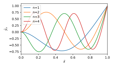
Modelling fluids
Our fluids can generally be expressed with the navier stokes equal which models
ρ[∂t∂u+(u⋅∇)u]+∇p=f+μ∇2u
This is a momentum equation
f is external volumetric force
Non dimensionalising NS
We can non dimensionalise the navier stokes equations, for turbulant flows relevant length scales are:
u=Uu~ rescaling with a free stream velocity
ℓ=μ/(ρU) this is basically assuming constant reynolds = 1, for length scaling. In turbulent regime flow isn’t very Re dependant
p=ρU2p~ scale with dynamic pressure
f~=fL/ρU2 scale with dynamic pressure and length scale
thus we get:
UTL∂t~∂u~+(u~⋅∇~)u~+∇~p~=f~+Re−1∇~2u~
Differences between low reynolds and high reynolds flows.
Low reynolds flow
Here viscosity completely dominates inertia, so our acceleration term and material derivative term can be removed, this leaves:
−∇p+μ∇2u=f These are the stoke equations
This is linear
no du/dt term so it is instantaneous
reversible (fluid can be unmixed)
High reynolds flow
this is generally the flow regime of our everyday life with big objects moving at high speed.
Inertial forces dominate over viscous forces and flow can almost be considered inviscid
Except in a boundary layer where viscous effects dominate
We can model many important results in terms of inviscid potential flow + a boundary layer effect
High reynolds example: Thin airfoil lift
An example of high reynolds flow is thin airfoil lift
This is completely modelled with potential flow theory, where we are examining flow over a spinning cylinder
Now remapping this flow where the cylinder turns into a flat plate using a joukowski transform
The vortex we are using to model contains the vorticity that would be carried within a boundary layer in the real world.
This leads to the result:
FL=21ρU2cCL(α,Re),whereCL(α,Re)≈2πα,
This predicts no drag (D’alembert paradox) boundary layer theory is needed to model this, with drag being shown to be
FD=21ρU2cCD
High reynolds example: Bluff body
1. The Breakdown of Potential Flow
In potential flow theory, a fluid is assumed to be inviscid and "slip" perfectly around a body, meeting up again at the back to recover the pressure. This leads to D'Alembert's Paradox, where the math predicts zero drag because the front and back pressures cancel out.
Separation: For bluff bodies, the high Reynolds number flow cannot handle the "climb" against the increasing pressure on the back half of the shape.
Vorticity Shedding: The boundary layer detaches (separates), shedding vorticity into the region behind the body.
The Wake: This separation creates a wake—a region of low-pressure, turbulent fluid that prevents the pressure recovery predicted by potential flow.
The wake is very unsteady, but we can average out the unsteadiness and define an average drag and lift:
FD=21ρU2ACD
FL=21ρU2ACL
Discussion of statistical steadiness
The parameter UT/L, defines how quickly our system changes. If it is large, it means our system moves slowly relative to the flow field
However: if it is small this our system moves at a similar speed to the flow field, no more spectral separation. this is the realm of our vortex induced vibrations.
Simplified NS example: Unsteady fluid carrying conduit
This is an example of how we can simplify the complex 3d navier stokes equations to 1D.
Physical explanation
We can see a flexible pipe, carrying a fluid with constant density and a constant velocity across the crosssection
The centreline of the conduit is defined by X(s,t)
Finding velocity
Our velocity is at magnitude U and in the same direction as X, hence our velocity is the material derivative of X
u=∂t∂X+U∂s∂X=(∂t∂+U∂s∂)X
Finding acceleration
Our fluid acceleration is defined as the material derivative of velocity
a=(∂t∂+U∂s∂)u=(∂t∂+U∂s∂)2X
Force on pipe
Now because the crosssection is uniform, and the fluid is inviscid, the pressure is constant. As such the only force on the pipe is from the fluid acceleration.
F=−ρAa=−ρA(∂t∂+U∂s∂)2X
Examples
now considering two examples
Semi circular conduit
here we are considering a steady conduit with square side b, it forms a quarter circle with radius R
There is a centrifugal force on the conduit at the 45 degree direction
Can solve easily by considering inlet and outlet momentums
If you hate yourself you can do the integral of force along the length
Flexible conduit
Here we have a pipe which the centreline is varying sinusoidally given by X=se^x+aℜ(eiωt−iks)e^y
Using our force function, our force per unit length is F=ρAa(ω+kU)2ℜ(eiωt−iks)e^y
Can see that we have an amplifying force that can result in instability
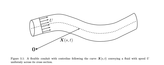
Simplified NS example: Thin layer flow
Now we are considering a thin layer of fluid which is viscous but incompressible. Our goal is to find the fluid pressure to find the force on the wall.
Mass continuity
First our fluid is incompressible so we can add teh condition: ∂t∂h+∂x∂q=0,whereq=∫0hu(x,y,t)dy
Considering extreme viscosity cases
We can consider two limits for our navier stokes equations, our euler equations which are inviscid and our viscous dominated stoke’s equations
Viscous case
Now our fluid is dominated by viscosity, so our navier stokes reduces down.
ρ[∂t∂u+(u⋅∇)u]+∇p=f+μ∇2u (no momentum transport terms and no external force), we are left with only pressure and momentum diffusion
∇p=μ∇2u
in 1D this is: ∂x∂p=μ∂y2∂2u⟹u=−2μ1∂x∂py(h−y)
this is our poiseuille profile
Inviscid case
Now we neglect our viscous terms so navier stokes goes to the euler equations
ρ[∂t∂u+(u⋅∇)u]+∇p=0
We need to guess the velocity profile, a common guess is a top hat profile ie q=uh.
We can use euler equations directly to find our pressure (or unsteady bernoulli which is derived from euler)
Example, onset of roll waves.
We have a thin film of fluid rapidly flowing down at an incline θ, this forms an undulation at the surface. Determine the onset criteria for these undulations
Assumptions
Since it says rapidly, we can approximate our fluid as inviscid
We will take wall drag as the Chezy friction coefficient: d(u,h)=Cfρhu2
plugging into governing equations
Continuity transforms to: ∂t∂h+∂x∂(uh)=0
Navier stokes goes to: ∂t∂u+u∂x∂u+gcosθ∂x∂h=gsinθ−Cfhu2
Linear stability analyisis
Now lets consider our perturbations:
u=U+u’ and h=H+h’
plugging this into navier stokes and removing small terms, we get:
∂t∂h′+U∂x∂h′+H∂x∂u′=0
∂t∂u′+U∂x∂u′+gcosθ∂x∂h′=Cf(H2Uu′−H2U2h′)
Now solving for normal mode solutions in form (u′,h′)=(u^,h^)esteikx
we get:
sh^+ikUh^+ikHu^=0
su^+ikUu^+gcosθikh^=gsinθ(2Uu^−Hh^)
At the threshold our real component is zero, so we are on the imaginary axis
looking at the real and imaginary components of the equation
we get the threshold:
gHcosθU2=2or, equivalently,tanθ=2Cf
This is the square of the froude number, showing how this non-dimensional quantity is relevant for fluid waves.
our stability is when we have a breakdown of friction as shown by the tanθ relationship
![<p>Now we are considering a thin layer of fluid which is viscous but incompressible. Our goal is to find the fluid pressure to find the force on the wall.</p><p><strong>Mass continuity</strong></p><p>First our fluid is incompressible so we can add teh condition: $$\frac{\partial h}{\partial t}+\frac{\partial q}{\partial x}=0,\quad\text{where}\quad q=\int_0^{h}u(x,y,t)\,dy$$</p><p></p><h3 id="4be93f90-9af3-4ce9-97f4-2cc2c406aeca" data-toc-id="4be93f90-9af3-4ce9-97f4-2cc2c406aeca" collapsed="false" seolevelmigrated="true">Considering extreme viscosity cases</h3><p>We can consider two limits for our navier stokes equations, our euler equations which are inviscid and our viscous dominated stoke’s equations</p><h4 id="292ba3d6-014e-46d2-a77f-0c66d4395748" data-toc-id="292ba3d6-014e-46d2-a77f-0c66d4395748" collapsed="false" seolevelmigrated="true">Viscous case</h4><p>Now our fluid is dominated by viscosity, so our navier stokes reduces down.</p><ul><li><p>$$\rho\left[\frac{\partial\mathbf{u}}{\partial t}+(\mathbf{u}\cdot\nabla)\mathbf{u}\right]+\nabla p=\mathbf{f}+\mu\nabla^2\mathbf{u}$$ (no momentum transport terms and no external force), we are left with only pressure and momentum diffusion</p></li><li><p>$$\nabla p=\mu\nabla^2\mathbf{u}$$ </p></li></ul><p>in 1D this is: $$\frac{\partial p}{\partial x}=\mu\frac{\partial^2 u}{\partial y^2}\implies u=-\frac{1}{2\mu}\frac{\partial p}{\partial x}y(h-y)$$ </p><p><strong>this is our poiseuille profile</strong></p><p></p><h4 id="4771dbf6-564e-41a1-88b9-24c571e3e8f4" data-toc-id="4771dbf6-564e-41a1-88b9-24c571e3e8f4" collapsed="false" seolevelmigrated="true">Inviscid case</h4><p>Now we neglect our viscous terms so navier stokes goes to the euler equations</p><ul><li><p>$$\rho\left[\frac{\partial\mathbf{u}}{\partial t}+(\mathbf{u}\cdot\nabla)\mathbf{u}\right]+\nabla p=0$$ </p></li></ul><p>We need to guess the velocity profile, a common guess is a top hat profile ie <span style="line-height: 1.15;">$$q = uh$$</span><span>.</span></p><p><span>We can use euler equations directly to find our pressure (or unsteady bernoulli which is derived from euler)</span></p><p></p><h4 id="9e0c3838-bbaf-469e-9b8c-d7e65c9af46f" data-toc-id="9e0c3838-bbaf-469e-9b8c-d7e65c9af46f" collapsed="false" seolevelmigrated="true">Example, onset of roll waves.</h4><p>We have a thin film of fluid rapidly flowing down at an incline θ, this forms an undulation at the surface. <strong>Determine the onset criteria for these undulations</strong></p><p><strong>Assumptions</strong></p><ul><li><p>Since it says rapidly, we can approximate our fluid as inviscid</p></li><li><p>We will take wall drag as the Chezy friction coefficient: $$d(u,h)=C_{f}\rho\frac{u^2}{h}$$ </p></li></ul><p></p><p><strong>plugging into governing equations</strong></p><ul><li><p>Continuity transforms to: $$\frac{\partial h}{\partial t}+\frac{\partial(uh)}{\partial x}=0$$ </p></li><li><p>Navier stokes goes to: $$\frac{\partial u}{\partial t}+u\frac{\partial u}{\partial x}+g\cos\theta\frac{\partial h}{\partial x}=g\sin\theta-C_{f}\frac{u^2}{h}$$ </p></li></ul><p></p><p><strong>Linear stability analyisis</strong></p><p>Now lets consider our perturbations:</p><ul><li><p>$$u = U + u’$$ and $$h = H + h’$$ </p></li></ul><p>plugging this into navier stokes and removing small terms, we get:</p><p>$$\frac{\partial h'}{\partial t}+U\frac{\partial h'}{\partial x}+H\frac{\partial u'}{\partial x}=0$$ </p><p>$$\frac{\partial u'}{\partial t}+U\frac{\partial u'}{\partial x}+g\cos\theta\frac{\partial h'}{\partial x}=C_{f}\left(\frac{2U}{H}u^{\prime}-\frac{U^2}{H^2}h^{\prime}\right)$$ </p><p>Now solving for normal mode solutions in form <span>$$(u', h') = (\hat{u}, \hat{h}) e^{st} e^{ikx}$$ </span></p><p>we get:</p><ul><li><p>$$s\hat{h} + ikU\hat{h} + ikH\hat{u} = 0 $$ </p></li><li><p>$$s\hat{u}+ikU\hat{u}+g\cos\theta ik\hat{h}=g\sin\theta\left(2\frac{\hat{u}}{U}-\frac{\hat{h}}{H}\right)$$ </p></li></ul><p></p><p><strong>At the threshold our real component is zero, so we are on the imaginary axis</strong></p><ul><li><p>looking at the real and imaginary components of the equation</p></li><li><p>we get the threshold:</p></li></ul><p>$$\frac{U^2}{gH \cos\theta}=2\quad\text{or, equivalently,}\quad\tan\theta=2C_{f}$$ </p><p></p><p>This is the square of the froude number, showing how this non-dimensional quantity is relevant for fluid waves.</p><p>our stability is when we have a breakdown of friction as shown by the tanθ relationship</p><p></p>](https://assets.knowt.com/user-attachments/d02075e1-dd19-456c-ae82-d07ec66f2a42.png)