biostats exam 2

sampling distribution

predict the population mean, plotting values

standard error

average of a sample difference to the true population average

small standard error

sample mean does a good job at estimating population mean

large standard error

sample mean does not do a good job at estimating population mean

sample size affect on standard error

increasing sample size decreases standard error

sample size increase for μ, σ, s, and 𝑦ത

μ and σ: do not change

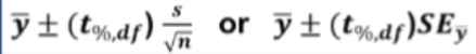
confidence interval

central portion of a standard normal curve, tells how many standard errors the sample mean is above or below the true mean

high confidence level

captures larger portion of the distribution but leads to false positives

low confidence level

produces narrower interval but with less certainty that the true mean falls inside it, more reasonable level of confidence

t distribution

replacement of s, adding uncertainty and creates a wider and heavier-tailed curved shape

certainty

how confident the interval is about capturing the true men, high CI = higher certainty

precision

reflects how tightly the interval pinpoints the true mean, lower CI = higher precision

sample size and CI

larger sample size = narrower CI

t distribution parameter

degrees of freedom, as df increases, T-distribution becomes more normal

degrees of freedom

n - 1, always round down

null hypothesis (H0)

claimed or assumed value of the population mean and serves as the baseline for assessing random chance

alternative hypothesis (H1)

competing claim and reflects the possibility that the population mean differs from the value stated in the null hypothesis

one sample t-test

uses data from one sample to evaluate population mean, determine whether sample is consistent with claimed value

reject H0

data would be unlikely to occur due to random chance alone if the null hypothesis is true, hypothesized value falls outside confidence interval

failing to reject H0

data does not provide enough evidence to rule out the null hypothesis (does not claim true), hypothesized value falls inside confidence interval

rejection region

tail areas outside of confidence intervals

a

significance level, establish threshold for rejecting null hypothesis BEFORE data analysis

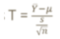
T*

measures how large the observed difference is relative to the expected sampling variability in units of SE, larger abs value of t* supports alternative hypothesis

p value

probability of obtaining a result at least as extreme as the one observed, assuming the null hypothesis is true

small p-value

more likely to reject null hypothesis (indicates observed data is unlikely to occur if H0 is true)

large p-value

fail to reject null hypothesis

p-value to a

p > a is fail to reject H0

P <=a is reject H0

type I error

false positive, test detects a difference even no difference exists, uses a probability

type II error

false negative, test fails to detect a difference even though a difference exists, uses B probability

role of a for type I/II error

a is larger, rejection region is greater, type I error increases and type II error decreases

t* compared to critical value

if t* is within central portion of distribution, fail to reject null hypothesis
if t* falls in the tails, null hypothesis is rejected

t-table

gives critical value, needs a and df

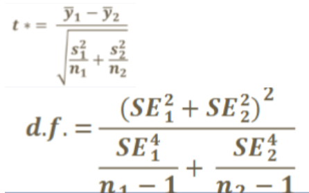
two-sample t-test hypotheses

null hypothesis: no real difference in the average value of the two populations
alternative hypothesis: population means differ

welchs t-test

useful for when groups have different variability

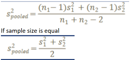
classic t-test

used when populations have similar variability, uses pooled variance

power

probability that the test will detect a difference when it exists, higher power is better at identifying it than missing, avoiding a type II error (1 - B)

power effects

increasing sample size, a (less strict a) and effect size increase power

classic test power

has higher power when population variances are the same

welchs test power

more powerful when unequal variances are assumed

three core assumptions

data collected randomly, two samples are independent, sample distributions are approximately normal

random data

reflect population in a fair or unbiased way, violated if a pattern is chosen out of convenience

independence

observations aren’t linked to each other, violation would be they dont function are seperate pieces of information

normality

samples come from normal distribution, violated if does not follow normal distribution

central limit theorem

increasing sample size can make data look more normal

histogram test for normality

gives a broad view for normal distribution

histogram limitations

depends on bin width, small size can lead to unevenness, may not show outliers

boxplot test for normality

shows summary for distribution center

boxplot limitations

broad summary, interpretation can be subjective

q-q plot

compares quantiles of the dataset to quantiles of theoretical distribution

quantile

cutoff value that divides a dataset into equal portion

normal q-q plot

straight line that runs diagonally from bottom left to top right of the plot

skewed left q-q plot

points start below reference line on the left side and rise above the line as you move to the right (long tail on the left)

skewed right q-q plot

points start above reference line on the left side and go below the line as you move right, then move up, (long tail on right)

short tails q-q plot

points lie alone reference line but show a dip below it, indicating fewer extreme values than expected (S - shape)

long tails q-q plot

points diverge from line, curve upwards at both ends, indicating more extreme values (backward S-shape)

mann-whitney U-test

used to compare two independent groups when data cannot be assumed to be normally distributed, appropriated when one group doesnt follow normal distribution

mann-whitney test assumptions

independent and random data (does NOT assume normality)

mann-whitney hypotheses

null (H0): distribution/mean of s1 is same as distribution/mean of s2 (D1 = D2)
alt (H1): distribution/mean of s1 is not the same as distribution/mean of s2 (D1 = D2)

U*

counting how many observations are smaller as 1 point, if equal than count as 0.5 points, k1 is count of the first sample, k2 is count of the second sample

U statistic

higher count of k, if tied, take average

MWU vs t-test

MWU does not require normality, t-test is more powerful if normality is assumed

paired t-test

used for dependent observation, assumptions are random data and normality, d = difference

paired t-test hypotheses

null hypothesis (H0): ud = 0, no difference between the observations in each pair
alt hypothesis (H1: ud =/ 0, difference between the observations in each pair

t*

t* > 0, average difference is positive

t* < 0, average difference is negative