AP Ch 6 CAPM & Portfolio Theory

two fund separation theorem

where lending/borrowing at the risk free rate allows me to exist outside the efficient frontier. ideally would split the funds into 2, one for a risk free asset and the other for the risky/market portfolio to optimize the portfolio

CML graph

represents all the portfolios that optimally combine the risk free rate of return and the market portfolio of risky assets

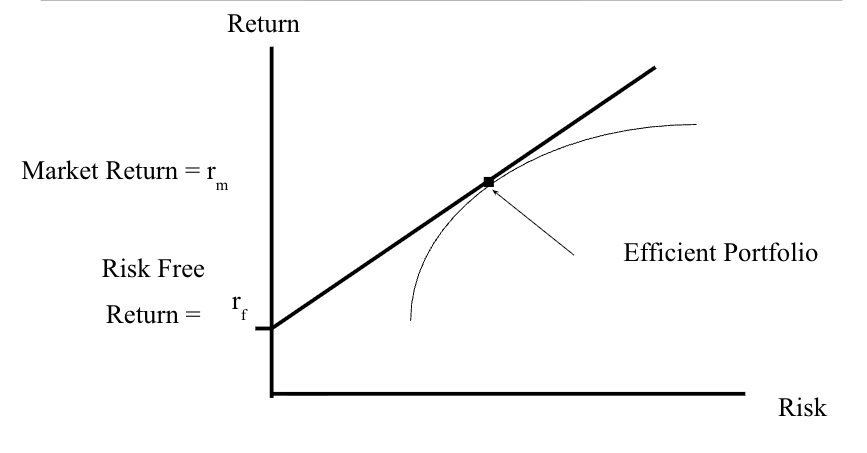
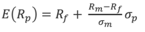
formula for CML when checking if a portfolio is efficient enough to lie on it

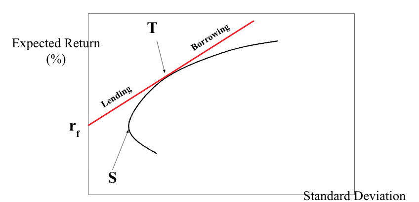
lending segment of the kinked CML

connects the risk-free asset to the market portfolio, representing investors who allocate some portion of their portfolio to risk-free lending. The slope of this line is determined by the risk-free lending rate

kinked CML

happens when the lending and borrowing rates are different as then the single CML is replaced by two separate lines that meet at the market portfolio. the borrowing line has a lower slope than the lending line because borrowing rates are typically higher than lending rates. so risk is lower when borrowing

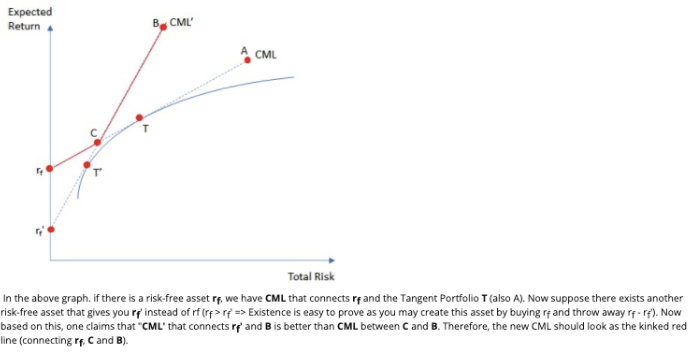
borrowing segment of the kinked CML

extends from the market portfolio, representing investors who borrow at a higher rate to finance additional investments in the market portfolio. The slope of this line is lower than the lending segment's slope due to the higher borrowing rate

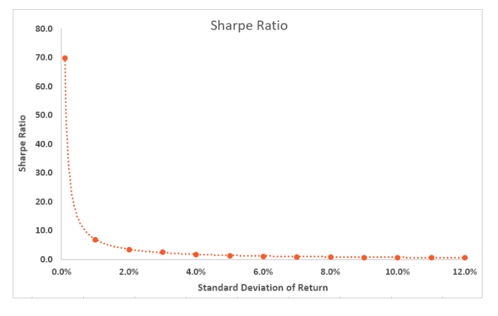
sharpe ratio

measures an investment's risk-adjusted performance by calculating the excess return per unit of volatility. when the overall risk has increased, the more favorable the portfolio is as there is an increase in rewards. however is the level of risk is unacceptable, it could be rejected. sharpe ratio = (expected return - rfr) / std

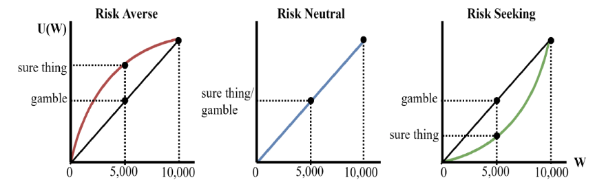
risk aversion

a preference for a certain outcome over a risky one with the same expected value. risk-neutral individuals have a linear utility function, while risk-seeking individuals have a convex (upward-curving) utility function

risk averse, neutral and seeking graphs

shows decreasing marginal utility from wealth. the greater the concavity of the function, the higher the degree of risk aversion

types of risk

• Firm-specific risks – business and financial

• Shareholder-specific risks – interest rate, liquidity, market

• Firm and shareholder risks – event, exchange rate, purchasing power, tax

return

total gain or loss experienced by an investor over a period (day, week, month , year etc)

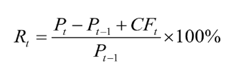
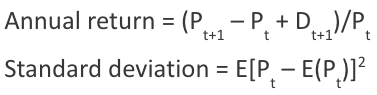
annual return and standard deviation formula

p is price and d is dividend

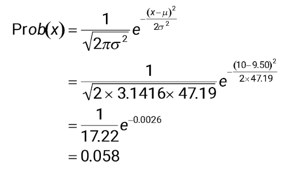
probability density function

used to find the probability of any return outcome

portfolio theory says risk can be diversified if

• assets are not all perfectly correlated with each other.

• a large number of assets are combined in a portfolio

efficient frontier

portfolios created with different weights on each assets lie on a smooth curve

portfolio

a collection of asset holdings. imp things to consider for it is weights, return and variances

equally weighted portfolio

every stock is allocated the same amount of funds and has the same portfolio weight

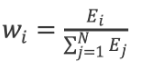
value weighted portfolio

each stock is assigned a weight equal to its market value divided by the total value of all stocks in the portfolio

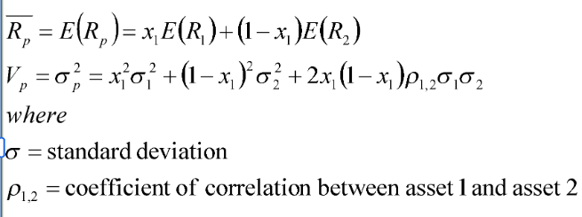
expected return and variance for a portfolio with 2 assets

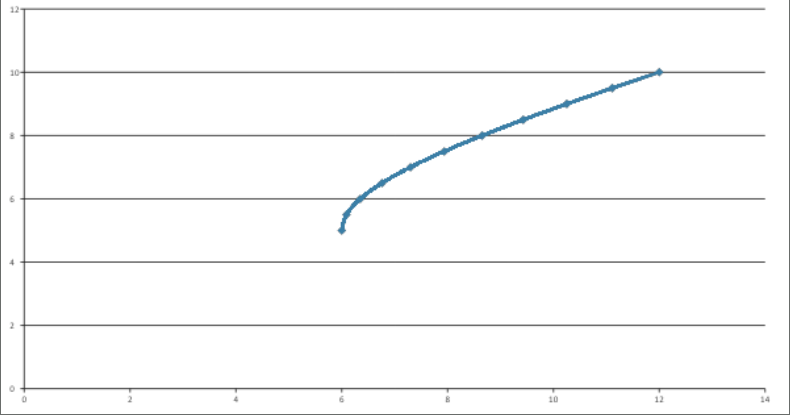
covariance and correlation formulae

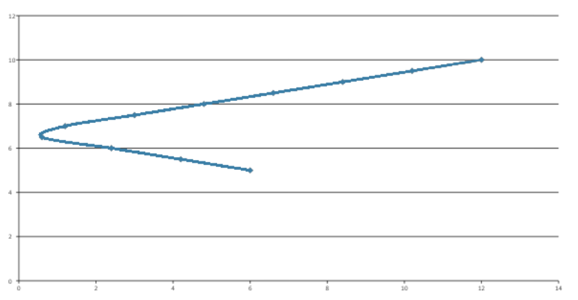
graph for stocks with no correlation

it’s flatter as the horizontal stock doesn’t really change or impact the vertical stock

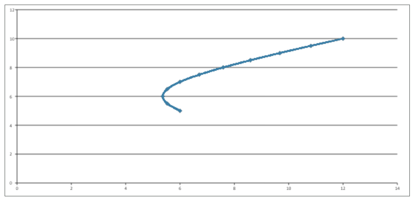
graph for stocks with perfect negative correlation

is in a v shape cus asset A and B are perfect hedges for each other and can offset each other perfectly. so it's starts at 100% asset A, moves towards the vertex near y axis where there's min risk and variance and then moves back out to 100% asset B

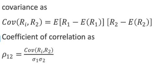
graph for stocks with less than perfect correlation

it's got this shape due to diversification reducing risk (std) without proportionally reducing expected return, making there be a delayed effect between the two and an imperfect correlation

relationship between variance and the coefficient of correlation

variance is smallest when the correlation coefficient is perfectly negative (-1) and largest when it's perfectly positive (+1)

diversification formula for expected return and variance for each stock

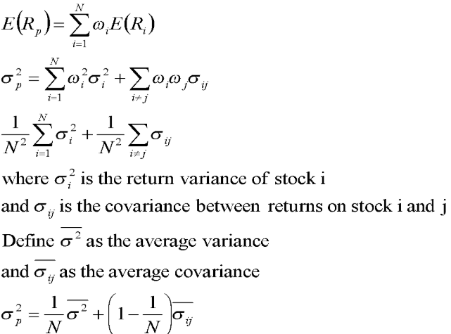
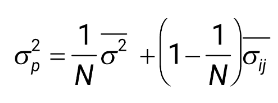
variance of an equally weighted portfolio

when N is sufficiently large, the first term disappears, leaving the portfolio variance equal to the average covariance between stocks

sum of covariances /N²

Average covariance x (N² – N)/N²

number of covariances in a N stock portfolio

N² – N

what to consider for for effective diversification,

• investors should have no preference between upside and downside risk

• the assets combined should not be perfectly correlated otherwise there will be a low correlation

• the number of stocks in the portfolio should be large

diversification and portfolio risk

combining more securities reduces the overall portfolio risk

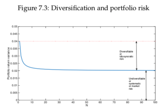
graph showing the relationship between diversification and portfolio risk

shows the standard risk goes down when the number of securities increase (more diversification)

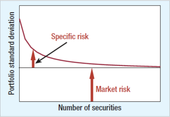
market risk

economy-wide sources of risk that affect the overall stock market, also called systematic risk

specific risk

risk factors affecting only that firm. also called diversifiable risk

diversification

strategy designed to reduce risk by spreading the portfolio across many investments

why introducing short selling is good

as it allows investors to take positions on negative portfolio weights, giving them more opportunity for profit

how to short an asset

• first borrow the stock from a broker

• then sell it when it's falling in price

• after a month or so you go buy that stock and return it to the broker, initiating and closing your short position

• if sold at a higher price you will make a loss

portfolio weight formula

final amt / initial amt, when shorting, the amt you're selling is considered negative

common utility function for investors

U = E(R) - 0.5AV, where A is the risk aversion coefficient and V is the variance (volatility measure)

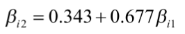
blume equation for adjusting betas

in the forecast period it lowers the beta value of a high value stock, making it less volatile and more stable while increasing the beta value of a low beta stock, making it more volatile than the overall market

why there can be estimation errors from beta changes (think mean reversion)

• estimation errors can be pos or neg

• predictive value for estimated beta based on historical data, but historic data is not necessarily better than a naïve assumption

• if the estimated beta > 1, positive error

• if the estimated beta < 1, negative error

• on average it tends to converge to 1, the market’s overall volatility level

limitations of estimating betas

• usual regression models don’t capture the time changing nature of beta

• there’s a higher random error for single securities than a portfolio of them due to the diversification effect

non-synchronised trading effect

when the return on a stock is not correlated with the return on the market

what equity market indices and bond indices do

measures the trends and returns on subsets of securities in each market such as stocks, bonds and options

4 things the estimated beta is sensitive to

• market proxies (e.g S&P 500, NASDAQ)

• measuring periods

• return intervals

• accuracy (stability and estimation error, measuring portfolio beta is more accurate)

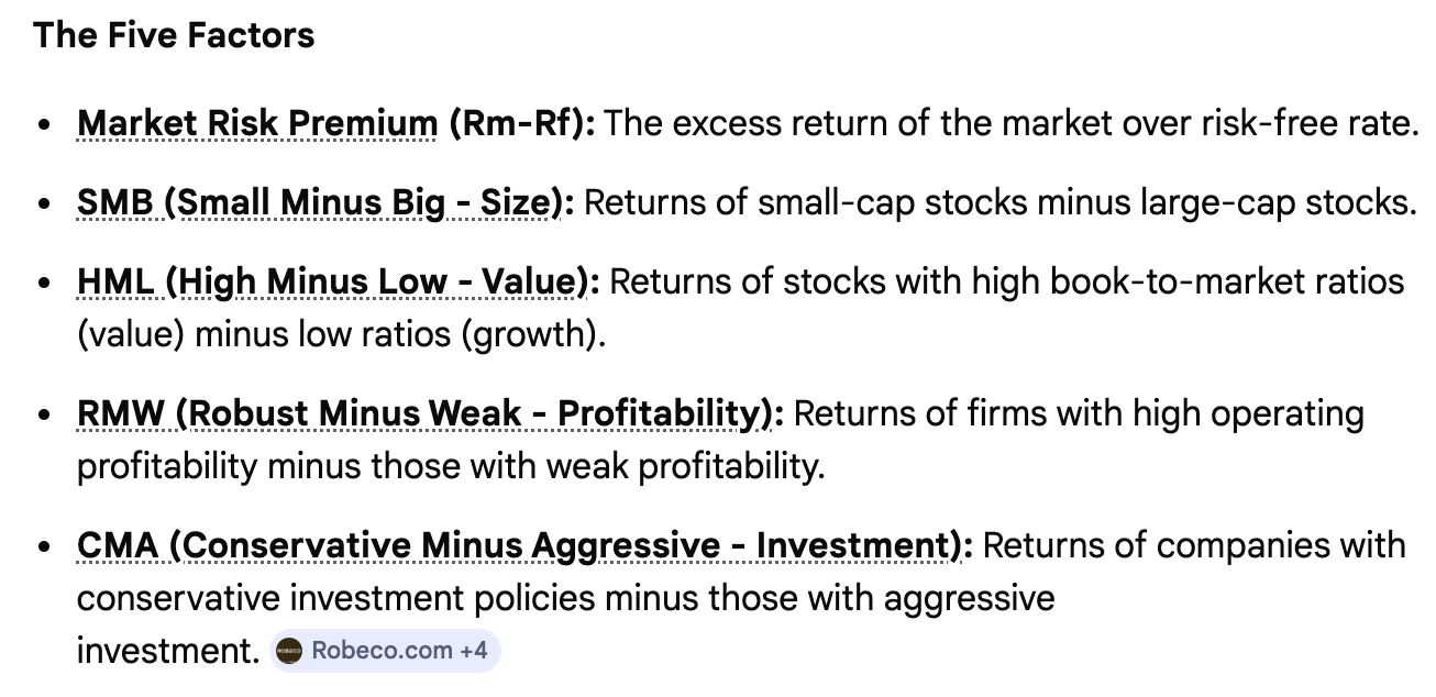
5 factor fama and french model

market, size, value, profitability, and investment

fama and french findings

even when market risk was controlled, smaller firm portfolios tend to have larger returns and high B/M (value) firms had larger returns than low B/M (growth) firms, so CAPM is rejected

double sort

categorizes stocks into portfolios based on two characteristics (e.g., size and book-to-market ratio) rather than one. analyzes the impact of these variables on returns and test if one variable's effect holds up when controlling for another

how fama and french was conducted

so to test it out accurately they split the six portfolios into 2 groups and randomly has one group be what's measured and the other be to construct the risk factors and then reverse it in the next trial

how the size and B/M risk factors are constructed

excess returns are regressed onto market returns, SMB and HML. this means to determine how much of the portfolio's outperformance is due to these factors using linear regression

what did fama and french include for the zero cost portfolio

SMB (long pos in small stocks and short pos in large stocks) and HML in market ratio (long pos in value stocks and short pos in growth stocks)

expected risk premium

expected return - rfr

macroeconomic factors affecting stock returns

interest rates, inflation, GDP growth, and exchange rates

examples of market risk measurements

yield curve or exchange rate

examples of macroeconomic risk

GDP growth or unemployment rate or inflation

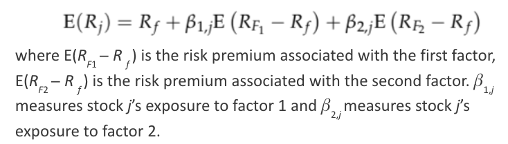
2 factor APT model

why APT is better than CAPM

CAPM only considers market risk while APT considers sensitivity and risk premium along with it also considers risk that affects the economic company prospects

assumptions for APT

• assets are generated from a k factor model (measure growth)

• no arbitrage opportunities

• no form specific risk after portfolio formation since enough assets are available

how to know the factor sensitivity of an asset

you need to know the asset's exposure to factors in order to replicate the returns

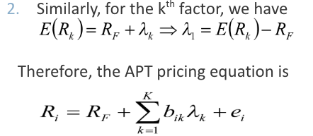
arbitrage pricing theory

used to compute returns

alternative models to CAPM

• arbitrage pricing theory (APT)

• multi factor models

• inter temporal CAPM

• consumption based asset pricing models (CCAPM)

what size says about expected returns

small stocks tend to have higher expected return than large stocks (holding β constant)

what value says about expected returns

mean returns on stocks with high book-to-market tend to be larger than those on low book-to-market stocks (holding β equal)

why should there not be any significant variation in average returns after holding beta equal

the returns will just follow the market beta and generate similar returns

what did fama and french do

• estimated beta values for each stock then organized them into 10 groups based on it

• then within these groups organized them by size and B/M ratio and then compared their average returns

• they did this to see whether market beta was a good indicator of average returns but it was not

• instead found the size and B/M ratio was also needed and so prompted them to create the 3 factor model

what does checking the residual form from the first pass do

basically checking if the risk from the years before affects the returns now through carried forward information

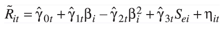
second stage CAPM test

produce a single cross-sectional regression for all assets by regressing the average historical return for each asset on the β for each asset

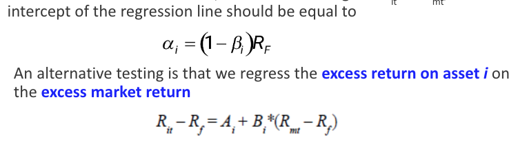
first stage test of CAPM

run a time series regression of that asset’s excess returns on the market excess return. if A doesn’t equal zero CAPM doesn’t work so well

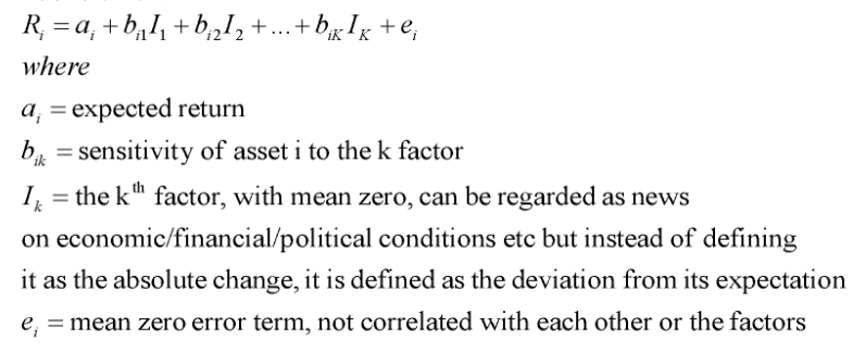
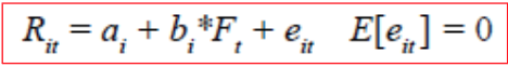
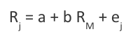
return of an asset

a is the asset specific constant, b is the asset specific factor sensitivity and e is the idiosyncratic variable uncorrelated across assets. f can be a factor common to the assets

why CAPM is and isn’t testable when the market portfolio isn’t observable

• the market portfolio is efficient but the chosen proxy isn't

• the market proxy is efficient but the market portfolio isn’t

• quality of the proxy is very important but can’t be guaranteed so results can’t really be trusted

what a true market portfolio can include

financial assets such as bonds and stocks and non financial assets such as real estate, durable goods and sometimes human capital

roll critique

a true market portfolio can't be reflected as non marketable assets can't be traded and therefore aren't included

how a short selling position is created

elling a call, borrowing an amount equal to the PV of the exercise price at the risk-free rate, and buying a put

what the put call parity implies regarding the risk free rate

a risk-free rate can be created by a stock, a call and a put

ex ante

before an event, making a prediction. ex post is the opposite

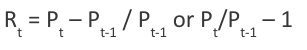
periodic return

today’s price – last period’s share price divided by the last period’s price

market portfolio

contains all marketable securities and assets, is unobservable and so a proxy is needed

beta estimation

regressing the returns on any asset j against the returns on a market index M (as a proxy for the market portfolio), over a reasonable time period

how to tell which is the riskier stock

riskier one is the one that has more systematic stock (beta) regardless of how much total risk it has

how to find the total risk of the asset

find standard deviation which you find by square rooting market variance which you find by  multiplying the probability by the difference between rate of return and expected return squared

how to find the systematic risk

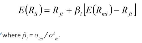
found by finding beta which is found by rearranging expected formula for expected return

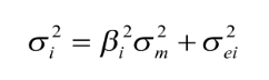
variance of an asset’s return

market variance = systematic risk + unsystematic risk

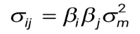
covariance of return between security A and B

beta A x beta B x market variance

unsystematic/diversifiable risk

only affects a specific sector, doesn’t affect expected returns, and is avoidable through diversification

systematic/undiversifiable risk

due to market movements, increases equilibrium expected returns and is unavoidable as it can’t be diversified

why in CAPM, random error is expected to be 0

as it's not correlated with the realized return or expected return on the market

why total return variances can differ even if their betas are the same

a proportion of asset return variance can be eliminated through diversification, diversifiable risk doesn't affect expected returns

3 applications of CAPM

• valuation of stocks, projects and portfolio selection.

• good for stock valuation as it can tell you what the expected returns are for the company's level of risk

• good for portfolio selection looks for the risk free asset and market portfolio combo that maximizes personal utility

when does CAPM say the market price is too high

expected return is below the CAPM expected return

when does CAPM say the market price is too low

expected return is greater than the CAPM expected return

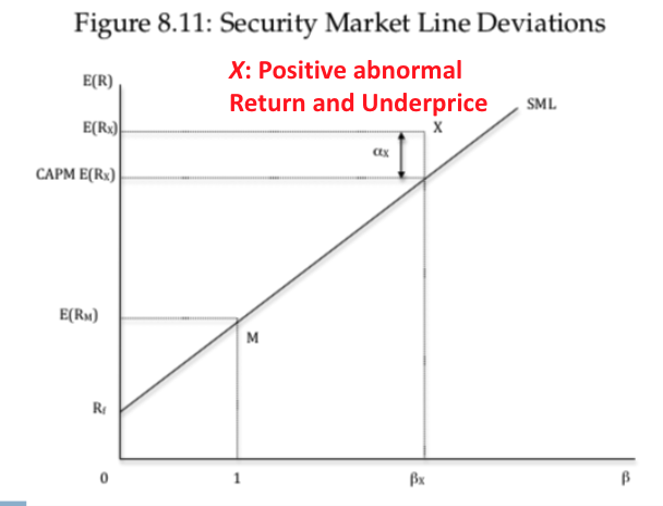
how to tell a stock is overpriced or underpriced using SML

when expected return is higher than the observed return and the stock lies above the SML it's overpriced. if it’s below the SML and expected return is lower than observed return it’s underpriced

how to get a positive abnormal return when possible

• create a portfolio with the market and risk free asset that has the same beta as stock x

• then buy stock x and short sell the portfolio.

• this will give a no risk arbitrage profit as there's a difference in the market and stock price.

• this will cause the stock x price to increase and restore equilibrium return on the SML

what it means for a stock that doesn't lie on the SML

it’s either overpriced or underpriced as otherwise when matching the market price, it’s on the SML

what happens if two stocks have different betas

a stock’s expected return would differ from the other

when beta < 0

negatively correlated with the market. the more negative the beta is, the more opposite movement to the market

when beta > 1

returns are positively correlated with the market return, asset is riskier than the market so return will be higher than the market's. when the market goes up by 1%, we expect the asset price to go up by more than 1% (in fact we expect it to rise by β %)

if beta < 1

it's still positive so the asset is risky but not as risky as the market and so the return will be less. when the market goes up by 1%, the asset’ price will go up by less than 1% (in fact we expect it to rise by β %)

covariance of the market

cov(R_i, R_m) = correlation coeff. x standard deviation of the asset x standard deviation of the market, needed to be divided by variance to find beta

when beta = 1

• has the same return as the market

• perfectly correlated with the market

• Cov(E(Rm), E(Rm)), must be equal to its variance, Var(Rm)

when beta = 0

the beta of a risk free asset as it has no correlation with the market or any asset in the market. has diversifiable risk

expected return when considering risk

shows return and risk are proportional