Inter-temporal macro

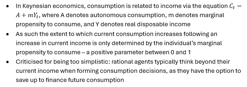
What is the Keynesian consumption function?

The intertemporal model of consumption can provide an alternative derivation of the IS.

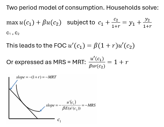
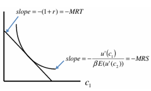
Derive the two-period model of consumption and show on graph:

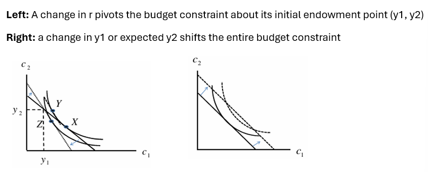
Show a change in R, and a change in y1/expected y2

How do we model the expected discounted utility in the future from now to infinity:

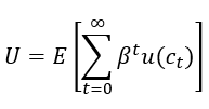
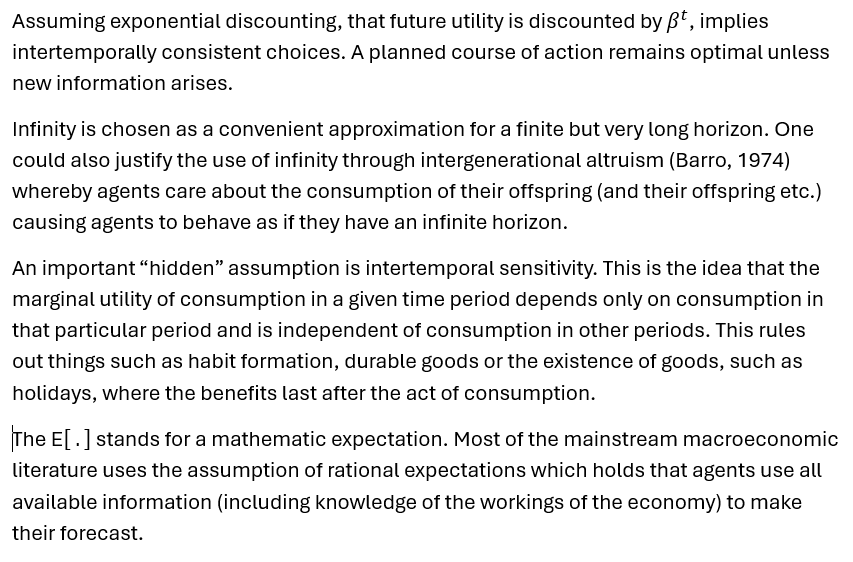
What are some assumptions in this equation?

What is the constraint?

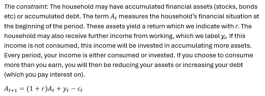
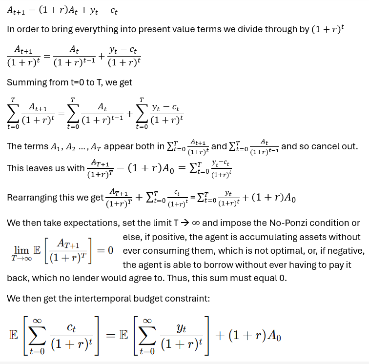
What is the intertemporal budget constraint:

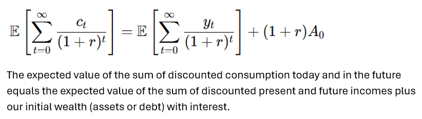
Derive the intertemporal budget constraint:

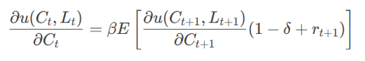
What is the Euler equation?

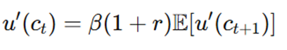
LHS is marginal utility of consumption in period t and RHS is the marginal utility of that same consumption at time t+1. If this condition did not hold then the original consumption in period t could not be optimal. If LHS < RHS, then a reduction in utility this period would be offset by a greater gain in utility next period. If LHS < RHS, it would be better to reduce next period consumption and increase consumption this period.

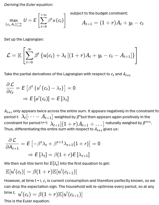
Derive the Euler equation:

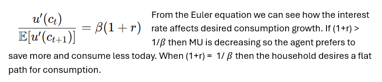
How does the interest rate affect desired consumption growth?

What is our first big assumption to get from the Euler equation to a consumption function?

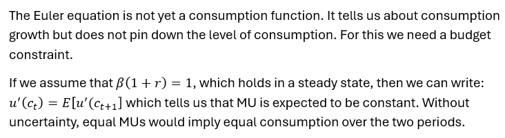
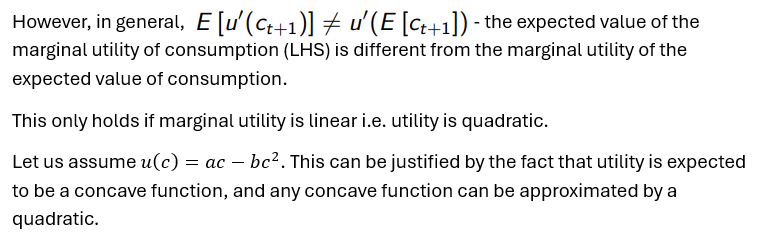
Does this hold, and what is our next assumption?

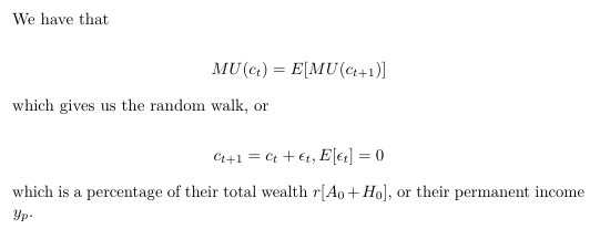
Derive the random walk hypothesis:

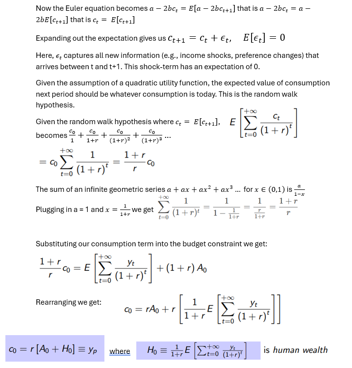
What does this tell us?

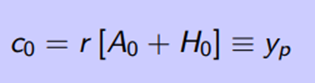
Now we have a consumption function that is a simple linear function of human wealth. The marginal propensity to consume out of total wealth is r.

This tells us that the timing of income does not matter. All that matters is the expected present value of income. Volatility of income does not affect consumption choices as, in choosing consumption, the household behaves as if future income were certain. This is known as certainty equivalence. If unexpected news about their income came in, the household would change their behaviour moving forward.

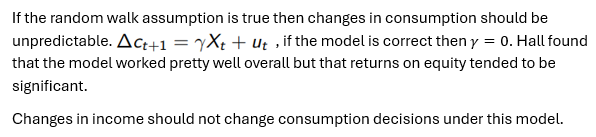
If the random walk assumption is true, then what should hold?

Proposed by Hall (1978), the random walk hypothesis postulates that all changes in consumption must be unanticipated

Borrows heavily from Friedman’s PIH:

• At any given moment consumer selects consumption based on their current expectations of their lifetime income

• Throughout their lifetime consumers constantly modify these decisions based on new information that makes them adjust their expectations

• Hence any changes made to income should not be affected by the arrival of anticipated changes in income, since if consumers are optimally using all available information, they should be surprised only by events that were completely unpredictable

• Hence consumption follows a random walk

What is excess sensitivity?

RWH predicts that changes in income that have been anticipated in advance should not lead to any shift in consumption levels at the time they actually occur, as agents should already have adjusted consumption levels immediately when information about the change is received

However it turns out that consumers do tend to exhibit a significant response (Flavin, 1983)

For example, a 2001 tax rebate in the US only led to a considerable increase in household consumption (by an average of 20%-40% of the rebate) when it was delivered, rather than when the programme was announced.

What is one explanation for excess sensitivity?

One explanation for this is credit constraints.

Zeldes (1989) also found evidence of excess sensitivity for credit-constrained households. Households will want to smooth their consumption to their permanent income level but, if their current income is below the level of permanent income, they will have to borrow to achieve it. However, if there is a constraint on borrowing then this level of consumption will be infeasible for the household.

While credit constraints can explain why households suddenly increase consumption when their current income rises (because they’re finally able to borrow against a higher permanent income), that mechanism doesn't clearly explain why households cut back on consumption just as sharply when their income drops. In theory, they should be able to smooth consumption in both directions—upward and downward—through borrowing and saving.

What equation does the agent use to predict income?

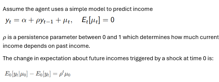
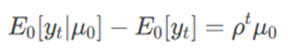
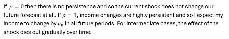
How does the value of p change things?

Derive the change to consumption:

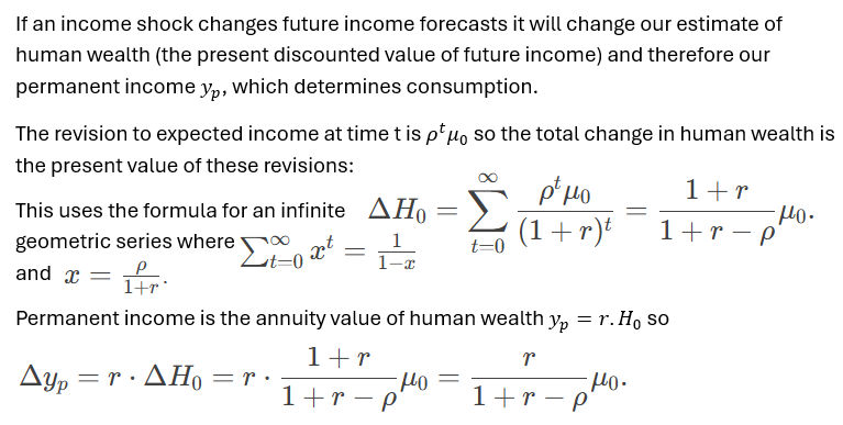
What does this tell us? What supports it?

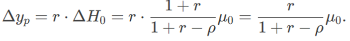
This tells us that the effect of a shock on consumption is larger the more persistent income shocks are perceived to be. Consumption responds more to persistent income shocks (e.g., promotions) than transitory ones (e.g., bonuses).

The Permanent Income Hypothesis (PIH) is bolstered by evidence that consumption responds rationally to income shocks based on their perceived persistence. Studies like Gelman et al. (2016) show households maintain consumption during transitory shocks (e.g., temporary pay freezes), aligning with PIH predictions. In developing economies, households save most transitory windfalls (e.g., good harvests), while adjusting consumption to permanent shocks (e.g., land inheritance), consistent with forward-looking behavior.

What is excess smoothing and sensitivity?

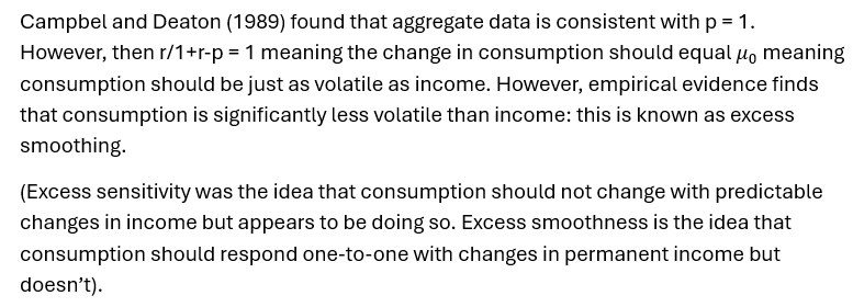
Excess smoothing (and excess sensitivity) suggest that our simple certainty equivalence model is missing something. Like what?

-            Liquidity-constrained households cannot borrow to smooth consumption fully, dampening responses to permanent shocks. It then leads to excess sensitivity when consumption responds to income changes more than PIH predicts.

-            Simultaneously, households may save more than the model predicts as a buffer against uncertainty, further contributing to excess smoothness. Recent evidence in support of precautionary saving was found in the 2024 American Economic Review which found strong evidence that uncertainty affected the spending choices of households.

-            If households derive utility from maintaining stable consumption over time (habit-formation) they may adjust consumption more smoothly in response to income shocks.

-            If households do not have perfect information or do not form expectations entirely rationally then consumption decisions may deviate from the predictions of the PIH. In particular, we may observe excessive sensitivity to (what should have been) predictable income changes.

Other problems with the model:

Furthermore, even if every single agent in the economy behaves as predicted by the standard model, when you look at aggregate consumption it does not respect the simple Euler equation. There is an aggregation problem.

Another strike against the standard model is the fact that, at the micro level, evidence suggests people do not always make time-consistent choices and instead exhibit present bias, choosing to consume more in the immediate present while postponing savings. This behavior contradicts the exponential discounting assumed where preferences remain consistent over time. However, this issue can be accounted for within the framework by incorporating hyperbolic discounting, which captures the tendency to overweight immediate gratification relative to future rewards.

Conclude this section:

In summary, with quadratic utility and perfect credit markets, consumption is a linear function of financial and human health. However, empirically – although we find some support for the model - we also find significant violations. The model can be brought more in line with data by including credit constraints and precautionary savings, along with relatively high discount rates.

What is there to say about other utility functions e.g. ln(ct)?

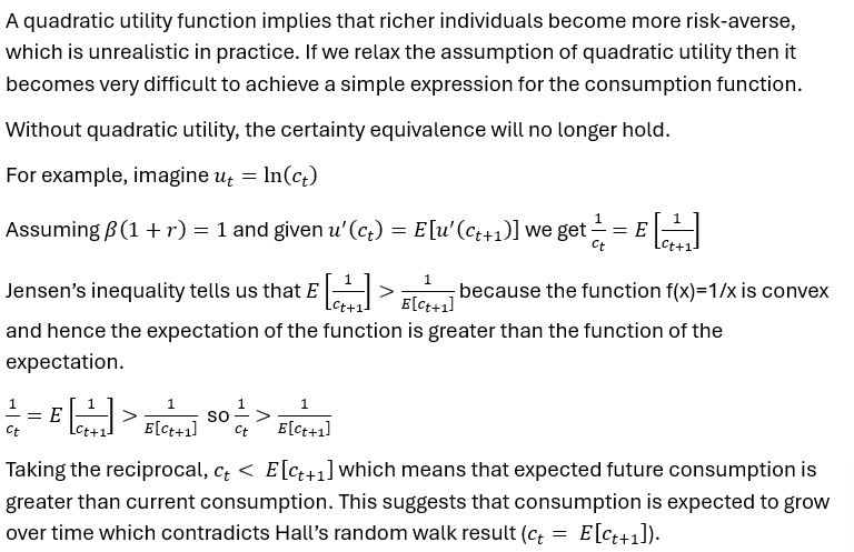
What explains excess smoothing?

The reason is precautionary saving: if we relax the assumption of quadratic utility, then the certainty equivalence result will no longer hold. Because future income is uncertain, it’s better to save some income now to guard against the possibility of future low income, which would give you less utility. And if people are indeed saving, then consumption is smoothed which gives us excess smoothness.

What is Ricardian equivalence, and what assumptions have to hold for it to be true?

Ricardian equivalence is the following claims:

• Government borrowing (debt finance) and tax increases (tax finance) are equivalent

• Debt-financed tax cuts have no stimulus effect

• A one-period government spending increase reduces wealth, but increases total output with a multiplier less than 1

These assumptions have to hold for Ricardian equivalence to be true:

• (PCM): Perfect capital markets: households can borrow at the same rate as governments

• (NCC): No credit constraints in the households

• (NPG): No population growth

• (NDWL): No distortionary effects of taxes (no deadweight loss, taxes must be lump-sum, taxes cannot increase future income)

• (STH): Same discount rate/time horizon amongst households and governments

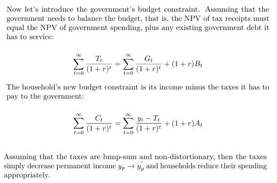
Summarise the household consumption side:

Introduce the government budget constraint and apply to consumption:

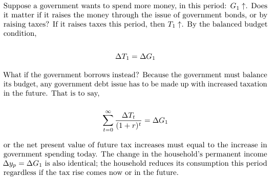
Show how government borrowing is equivalent to tax increases:

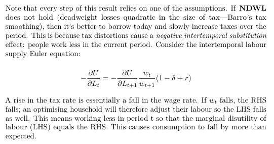
Why must NDWL hold?

Other assumptions:

Finally, if households have a different time horizon (STH) or the population is growing (NPG), then they would also rather the government borrow now and tax later, as the tax burden would fall less on them.

What are business cycles?

Business cycles are temporary and recurrent deviations of output and employment from the trend. Any economic variable can be decomposed into a smoother trend component and a (more volatile) cyclical component. A contraction is any period with a negative cyclical component.

What are the assumptions of our business cycle model?

Our business cycle model combines the long-run neoclassical growth theory (the Solow model) with short-run intertemporal models of consumption and investment. Key assumptions:

-            Savings are no longer constant, but instead consumers make decisions over their consumption and labour supply in order to maximize utility

-            Prices are flexible and the market is perfectly competitive

-            Business cycles are mostly driven by supply shocks which occur due to the randomness in exogenous technological progress. These shocks are then propagated through the economy via the accumulation of capital stock.

-            Given a model with perfectly competitive markets and prices, there is very little scope for policy intervention.

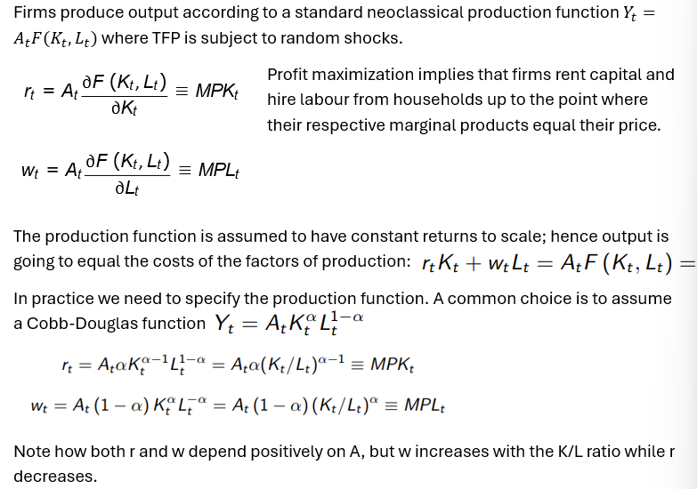
Explain the firm-side of the RBC:

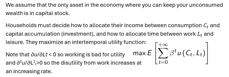
What must households decide?

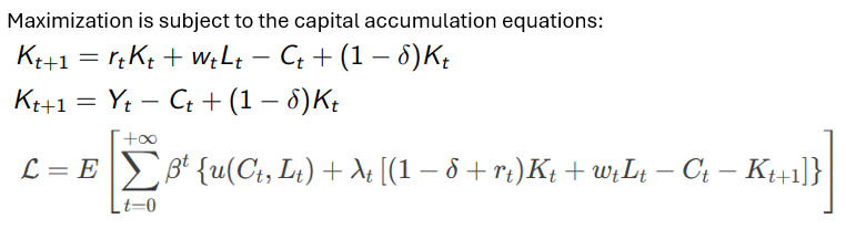
What is the capital accumulation questions, and the lagrangian?

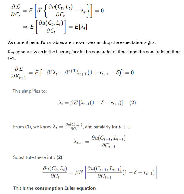
Derive the consumption Euler:

What does this tell us?

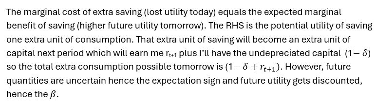
What about the intratemporal labour supply equation?

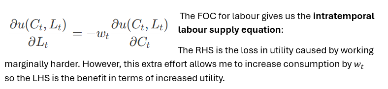
Derive the labour supply Euler equation:

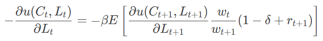
What does this tell us?

The equation balances the marginal disutility of labor today (left side) with the expected discounted disutility tomorrow (right side).

If I reduce work effort this period my utility increases by the marginal disutility of work. As I consequently earn less, I would save less, and end up with a lower capital stock at time t+1. To maintain the same level of Ct+1 and Kt+2 as originally planned I will have to work harder at t + 1. How much harder depends on the return to labour in the two periods and the return to capital in period t + 1.

In short, if wages are high today relative to expectations of future wages, I should work harder now and enjoy some pleasure next period.

Similarly, if I expect returns to capital to be unusually high next period, I will want to take advantage of that. Either I can consume a bit less in this period and save more or I can simply work a bit more which allows me to invest more. If the consumer prefers to smooth both consumption and leisure, they will do a little bit of both.

Where do business cycles come from?

What is the response to a shock where p = 0?

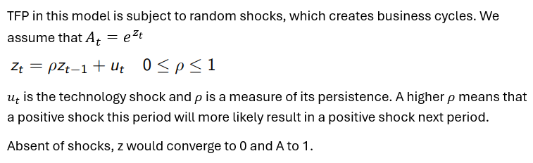
Starting from steady-state, assume a positive productivity shock in the initial period, so u0 > 0, so z0 > 0, and A0> 1 and . TFP is temporarily higher than the steady-state value (which is 1 here).

Given the rise in the marginal product of labour resulting from the increase in productivity, wages are pushed up temporarily. The household then faces an unusually high opportunity cost of leisure (substitution effect) alongside an income wealth effect which tells us we may want to enjoy more leisure.

In the real economy, we observe an upward trend in TFP but no downward trend in our work. To reflect this in the model, substitution and income effects must exactly cancel out for a permanent increase in productivity. An implication of this is that, in response to only a temporary productivity increase, the income effect is much smaller and therefore dominated by the substitution effect. This leads to an increase in the labour supply which amplifies the effect of the shock (we are more productive and on top of that, we are working more).

Greater productivity and labour input yields higher output which the agent must decide how to allocate. Given a desire to smooth consumption over multiple periods, the agent will increase consumption by a small amount today and save the rest of the higher output for the future. In fact, given that there are infinite future periods, only a fraction of the extra output will be consumed at time t=1; the rest will be invested leading to higher capital accumulation.

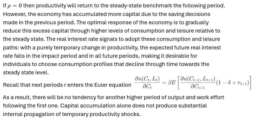
What happens next period?

<Skip> How do the different variables react under p = 0?

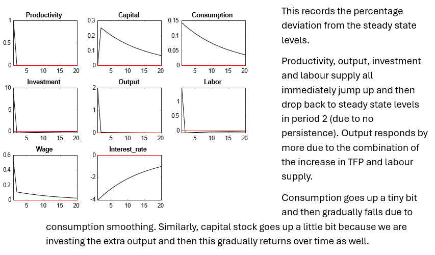
Which variables have a protracted adjustment?

When p=0, protracted adjustment can be observed for some variables, notably consumption, but otherwise we get very short cycles. Most variables return to steady state pretty quickly which does not match the volatility of these variables observed empirically. There is no close correlation between output and consumption that we see in the data.

The “fix” is to assume that technological shocks are highly persistent i.e. p > 0. In fact, to match the data well, the standard RBC model requires a value of  very close to 1.

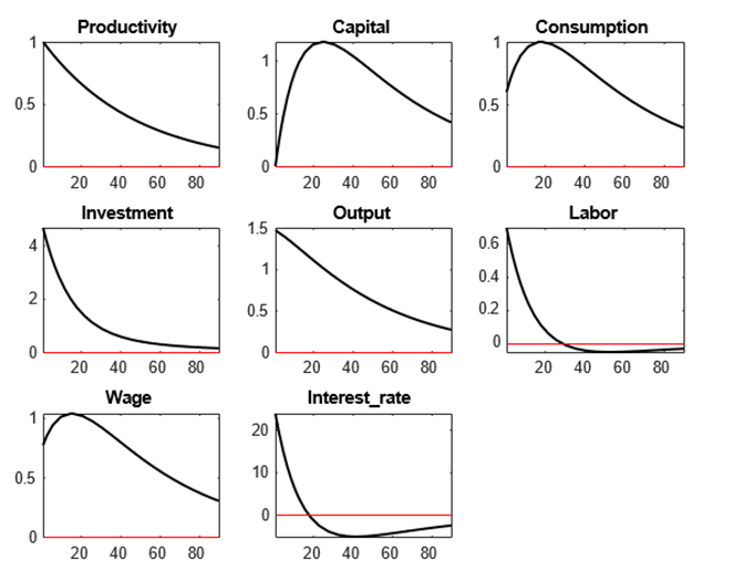
What changes with persistence? Start with capital and consumption:

With persistent technology shocks, the same mechanisms are at work but these effects are now drawn out over time.

Capital initially increases as higher productivity raises the marginal product of capital (MPK), incentivising more investment. Since productivity remains elevated for longer, this effect is sustained — capital keeps accumulating for many periods. Over time, however, the diminishing returns to capital set in, and as productivity eventually falls, the capital stock also begins to gradually decline.

Consumption jumps immediately due to the wealth effect: households anticipate a longer period of higher income from both wages and returns on capital. This expectation allows for stronger consumption smoothing over time.

What about interest rates?

Initially, the interest rate rises, as the MPK increases with higher productivity and investment demand spikes. But as capital accumulates and the MPK starts falling (due to diminishing returns), the interest rate begins a downward trajectory. Eventually, as productivity dissipates but capital remains temporarily above steady-state, the interest rate undershoots — falling below its steady-state level during the adjustment phase. This reflects a hangover from excessive capital accumulation even after the productivity boost from the shock is gone.

What about Labour supply?

Labour supply increases on impact due to the substitution effect (higher real wages encourage more work). However, this effect is dampened somewhat by a stronger wealth effect, since workers anticipate persistently higher future income. This causes labour to rise by less than it might under a transitory shock. As a result, the magnification effect on output is also slightly smaller. Over time, labour supply gradually returns to its steady state, dipping below the steady state level because the substitute effect wanes (wages are returning to steady state level) but there is a strong wealth effect (due to higher capital) which makes the agent want more leisure and also a low real interest rate which discourages work effort (see the labour supply Euler equation).

Graphs for variables:

Are business cycles good? Does the data fit?

Despite optimal responses from firms and agents, this is not to say that business cycles are a good thing. However, given that we cannot eliminate shocks to technology, this business cycle response is optimal and therefore there is no need for stabilisation policies.

Comparing our model to data collected by King and Rebelo (1990) it is a fairly close match, especially for a relatively simple model. However, wages are very strongly cyclical in the model but not so much in the real economy. Furthermore, the real interest rate appears to be cyclical in the model when, in the real economy, it is counter-cyclical. Given the importance of factor prices in guiding the agent’s decisions in the model, this is quite worrying.

What about aggregate demand shocks?

Aggregate demand shocks are not found to give plausible results in this framework. For example, agents know that an increase in government spending has to be financed sooner or later by taxes, causing the present value of after-tax income to fall. This would cause households to cut consumption and increase labour supply, causing output to rise. Thus, if government spending were the only shock in the model, consumption would be countercyclical which is contrary to the data.

Similarly, changes in labour and capital income taxes do have effects that are similar to productivity shocks and therefore could create business cycle fluctuations that match with the data. However, these taxes change infrequently making them poor candidates for sources of business cycles fluctuations.

Hence, this is why most economists tend to focus on supply side shocks.

What is there to say about labour supply elasticity?

The RBC model also need to align the empirical realities that real wages are, at best, mildly pro-cyclical but labour supply is very strongly pro-cyclical. With the assumption of a perfectly competitive labour market, the model requires a very elastic labour supply. However, micro evidence indicates that labour supply is not actually very elastic, and this has been a major criticism of RBC models.

Can the RBC resolve this?

This paradox is resolved by recognising that fluctuations in aggregate labour supply often reflect changes in employment status — people moving in and out of jobs — rather than adjustments in hours worked by those already employed. While individual workers may be reluctant to adjust their hours due to fixed schedules or contracts, they may be highly responsive in deciding whether to work at all. This allows aggregate labour supply to respond strongly to economic shocks even if individual labour supply appears inelastic.

Furthermore, long-term contracts act as implicit insurance: workers accept stable wages across the cycle, working more in booms without large pay rises in exchange for fewer wage cuts in recessions. This helps explain why wages appear less pro-cyclical in reality, despite strong movements in labour supply.

The key point is that going beyond the simplest labour market model and introducing more realistic features, for example that individuals may have limited choice on the number of hours worked, could resolve the labour elasticity problem.

The modifications still imply that, to the extent that there is a fall in labour supply during a recession, this additional unemployment is largely voluntarily which seems to be a weak spot of the analysis.

Conclusion on the RBC:

In conclusion, the RBC model presents a coherent approach to analyse macroeconomic fluctuations. Even its simplest version is remarkably successful at replicating some key movements observed in the data, but some aspects of the models are problematic (particular regarding factor prices). It is however a very flexible framework, in the sense that some of the most unrealistic assumptions can be relaxed without fundamentally altering the key findings.