Data Structures & Complexity

String Matching Algorithm

Algorithm to determine if a pattern (substring) of length m exists in a given text of length n. Finds valid shifts.

Has a naive algorithm which has O((n-m-1) * m) running time

Has KMP algorithm which has O(m) preprocessing and O(n) running time.

x is a prefix of y

x ⊑ y

x is a suffix of y

x ⊒ y

Suffix Function

Used (indirectly) in KMP algorithm. For a given pattern P, computes the length of the longest prefix in P that is also a suffix of the given string, x.

It tells us how many characters are currently matched and reusable at the end of the text scanned so far.

For the pattern P, |P| = m, let Q = {0, 1, 2, . . . , m − 1, m}.
σ : Σ∗ → Q by σ(x) = max{k : Pk ⊒ x}

Used in the DFA matcher, (Q, Σ, δ, 0, {m}) by δ(q, a) = σ(P_qa) for all q ∈ Q and a ∈ Σ. (P_qa is the prefix at q, plus new character to test).

If P = x it would return itself because there is no proper prefix requirement.

Prefix Function

Used in KMP algorithm. An application of the suffix function, with an extra condition that the whole overlap can’t be reused.

For a given pattern P, it computes the length of the longest proper prefix of P which can be reused, i.e a proper prefix of P_k that is also a suffix of P_q. Differs from the suffix function because it must be a proper prefix, so it can’t return itself.

π : {1, 2, . . . , m} → {0, 1, . . . , m − 1}

π(q) = max{k : k < q ∧ Pk ⊒ Pq }

Knuth-Morris-Pratt (KMP) Algorithm

String-matching algorithm used to find valid shifts via the prefix function (restricted offshoot of the suffix function).

• Compute prefix function (longest reusable prefix at each index). Use an index, q, to store backtracks.

• For each letter in the string T, compare it with P[q+1]

  • If T doesn’t match, hop backwards to the last valid prefix by doing q = π(q) repeatedly until match or q=0.

  • If T matches, increment q. If q = length of P, a match is found, record it.

• Record q = q+1 (i.e. if q was 0, record 1)

Abstract Data Type (ADT)

A collection of types, constants and operations performed on objects of those types, specified by characteristic identities.

Examples are a stack, queue, priority queue and dictionary.

ADTs are implemented using data structures. e.g. a priority queue is implemented using a binary heap.

ADT Priority Queue

A data structure that maintains a set of S elements, where each element has a priority. 2 implementations are binary heaps (heapsort) and binomial heaps (merge).

Types:

• E - Type of elements

• K - Linearly ordered type of priorities or keys

• P = P(E, K) - Type of priority queues (parameterised)

Constants and Functions:

• empty: P

• isEmpty: P → Boolean

• insert: P x E x K → P

• decreaseKey: P x E x K → P

• peek: P → E

• deleteMin: P → P

Binary Heap

An implementation of the priority queue ADT, which is a rooted, ordered binary tree with nodes with priorities, characterised by:

• Order - parent node priority >= children (if 1 = high priority then parent < child)

  • Shape - all layers are complete except the last, which is filled from the left

All operations are O(log n) except finding minimum, peek, O(1) and heapify, merge array, O(n).

Binomial Heap

An implementation of the priority queue ADT, which is a collection (forest) of binomial trees where each tree is in heap order, and there is only one of each order of tree. Faster merging.

All operations are O(log n) except check empty, O(1)

Binomial Tree

An implementation of the priority queue ADT which is a recursively-defined rooted, ordered tree.

B_k consists of two trees B_k-1 linked together, where the root of one is the leftmost child of the root of the other.

It always has 2^k nodes, with height k. The root’s children are binomial trees of decreasing order.

Binomial Tree node structure

• Degree

• Priority/Key

• Information

• Left child

• Right sibling

Linking 2 binomial trees

Must be same size.

Higher priority tree’s child becomes lower’s NEW sibling

Lower priority tree becomes higher’s new child.

Shift the higher child to become the sibling. Move over lower tree as child.

Merging binomial heaps

Recursively:

• If one root has smaller degree, keep it as the root, and merge its sibling with the other tree

• If both are equal degree, recursively merge remaining siblings, then link the equal-degree trees

Inserting element into binomial heap

Put element inside a new B₀ and then merge it.

Extracting the minimum value of a binomial heap

• If there’s only one tree, remove the root and merge the child and sibling.

• If there’s multiple, locate the top-level root with minimum value

• Reverse its children from being high → low order into low → high (for merging)

• Remove the root and merge the remaining trees

ADT Dictionary

An ADT made of a collection of key-value pairs, such that each possible key appears once from a linearly-ordered set. Can be implemented with hashing or search trees.

Types:

• K - totally ordered type of keys

• I - type of information

• D = D(K, I) - type of dictionaries (parameterised)

Constants and functions:

• empty: D

• isEmpty: D → Boolean

• member: D x K → Boolean

• lookUp : D x K → I

• insert: D x K x I → D

• delete: D x K → D

Hashing

An implementation of the ADT dictionary, where usually a small subset of keys are used.

Compute a hash function mapping keys to indices in the table, T, of size m.

Runtime for search, insert and delete are O(1) but collisions can occur and push to O(n).

Properties of a good hash function

Uniform distribution of used keys to buckets in the table.

Small change to key should create distinct and independent value.

Hashing Load Factor

For a table of size m, with n elements, indicates how full the hash table is with α = n/m

Types of hash functions

• Direct-address

• Chaining - Linked list for each slot

• Probing - Finding the next available slot

Hashing multiplication method

h(k) = m * (kA - ⌊kA⌋)

Take the decimal part and multiply by m (table size). Use an irrational number for A for uniformity.

Probing hash function

Mark slots with a flag: occupied, available or deleted (deleted continues search).

Use a hash function h(k, i), where the probing order is given by h(k, 0), h(k, 1),… h(k, m-1).

Linear probing

With a normal hash function h’, and i = 0, 1, .. m-1,

h(k, i) = (h’(k) + i) mod m

With collisions, slot probabilities change and become non-uniform. Leads to primary clustering.

Primary Clustering

Problem in linear probing where long clusters of occupied slots form, reducing efficiency as load factor approaches 1.

Quadratic Probing

With a normal hash function h’, and i = 0, 1, .. m-1,

h(k, i) = (h’(k) + c₁i + c₂i²) mod m

With collisions, slot probabilities change and become non-uniform. Leads to secondary clustering

Double hashing

Using a second hash function to determine the interval between probes. The second hash function should be independent of the first, and reach every slot so can’t divide m or be 0. More likely to yield uniform distribution.

h(k, i) = (h₁(k) + i * h₂(k)) mod m

In-order tree traversal

Traverse left subtree, current node, right subtree.

Binary Search Tree

A binary tree with the search tree property for every node:

• Nodes on the left subtree have smaller values

• Nodes on the right subtree have larger values

Operations are O(n) for member, lookUp, insertion and deletion because of no guarantee of list balancing. empty and isEmpty are O(1).

Deleting nodes from a binary search tree

• No children → Delete

• 1 child → Delete and connect parent to grandchild (linked-list style)

• 2 children → Replace with predecessor or successor

Red-black tree

Binary search tree where:

• Root is black

• No red node has a red child

• Black height is the same everywhere

• Null pointers are considered void black leaves

The height is at most 2x the black height, so any path can’t be more than twice as long.
A red-black tree with n internal nodes has height at most 2 log(n + 1).

Operations are O(log n) for member, lookUp, insertion and deletion. empty and isEmpty are O(1).

Black Height

The number of black nodes on any path from, but not including, a node x down to a leaf, denoted by bh(x).

Rotate red-black tree nodes right

Swap inner child, rotate clockwise.

The left node gives its right child to the right node.

Rotate red-black tree nodes left

Swap inner child, rotate counter-clockwise.

The right node gives its left child to the left node.

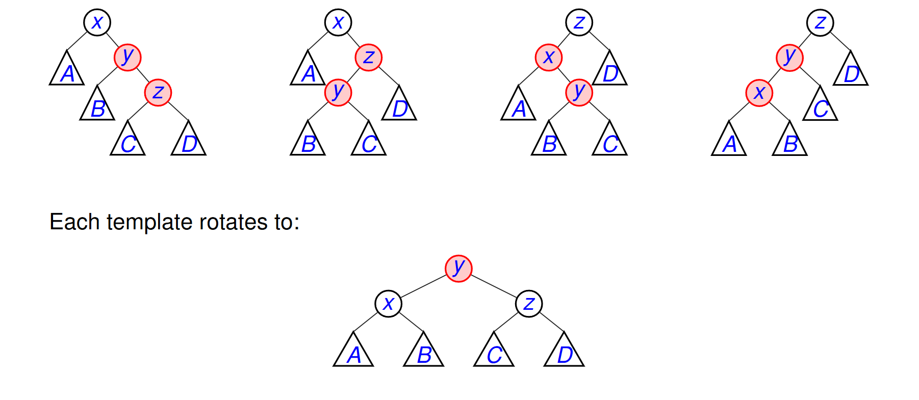
Matching red-red templates

Furthest-left is always x

Furthest-right is always z

Lower is always y

Each template rotates to xyz, where y is red.

Deleting black nodes adjacent to void leaf

Delete node, replace with child if able, else replace with NIL, donate blackness.

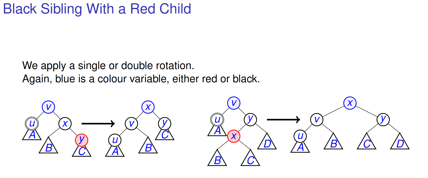
If it becomes double-black:

• Black sibling with red child - Rotate and recolour (propagate blackness up and try to absorb in the rotation, x takes v’s colour).

• Black sibling with black children - Push up blackness

• Red sibling - Rotate to a previous case

NOTE: double-circle node is the double-black NIL node after deletion