Multiple linear regression

how it differs from simple linear , Pop Equation + interpret constituents

• predict , model , observe changes in y from many x

1. Yi (the ith observation)= β0 +β1(slope parameter for the first x var) x1i(when the first x var is i (eg when x1 = 5) +β2x2i +...+βpxpi +ϵi

Correlation of multi linear regression

Correlation

• each x var with Y

• each x vars w each other

• Correlation matrix in R → make new object w just rows/columns you wanna look @ , cor function

Multicolinearity

a problem, thats why we check for it

• the correlated variables are both trying to explain the same variation in y - cant say which ones doing what. Causes UNCERTAINTY in parameter estimates

• Solutuion : Fit sepaerate models w only unrelated variables

Result of multicilinearity in regression analysis

• inflated standard errors leading to big p-vals

• big increase to RSE when adding a correlated x

• big changes to parameter estimates when adding/removing correlated x

Why does b0 in isolation sometimes not give useful info

this is the value when x=0 , x not really =0 for many real world things

interpretation of b hats

Bj → on avergae , the response var inc/dec by xxx for things for each additional unit xyz of explanatory var holding all else CONSTANT

B0 → Avg estimated Y val when all x vars = 0

Hypthoses test for significance on bj estimates

1. Same tstat from slr → EXCEPT df = t_(n-p-1)

2. R output

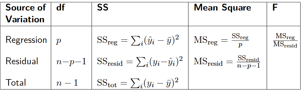
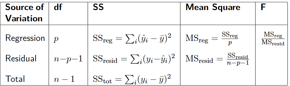
Checking overall model significance

1. H0 : no rlts btwn all x vars and y so ; B1 = B2= B2=…. = 0

H1: at least one Bj ≠ 0

2. F-stat → distribution Fp,(n-p-1)

…

3. Conclude : ….is/isnt linear rlts between at least 1 Bj var and Y

Adjusted coefficient of determination (R²)

More var we add to our model , less power/ability to detect a significant association cuz r² will stay same or increase when we add more x’s

so We use Adjusted R² = tweaked r² to account for sample size n no. x variables

Model checking

Same as linear BUT

• Check for independent errors → plot residuals against ALL x vars

1. Norm Q-Q Plot → normal dist errors

→ Linear rlts between

2. Hist(resids(model)) → Normality → Bell shape , Centred round 0 , symmetrical

3. Constant var → fitted vals vs residuals plot w red line → want randomn scatter round line

Categorical and binary variables

• Binary - has 2 levels eg Yes and No

• Binary → 0 and 1 (0 = reference category)

• Binary cat var → B4 (for example) represents change in Y when X4 is 0 or 1 -( Yes/No )

• B0 (intercept ) = effect on Y when X4 @ ref categorial ie when X4 is Yes

• In R = ref category is variable that comes first in the alphabet by default

1. Convert cat var to factor → data$column ← as.factor (data$column)

2. How to do it manually in R (choose own ref category) → slide 41

Cat var w/ More than 2 lvls (A,B,C) → still 1 Ref w/ Multiple B^ estimates capturing effect of dummy vars against ref category

Let A = ref;

^B5 → Change in Y when X4 is level B , vs when lvl A

^B6 → Change in Y when X4 is level C , vs when lvl A

Bj interpretations for categorical variables

B0 : on avg , y var is xyz when all x vars are zero AND all ref catergories are 0(according to their assigned categorical values)

B4(5…etc): On avg , y var increases/decreases by xyz for a one-unit increase in the corresponding x var, holding all other variables constant.

Categorical var → B5: On avg Y is xyz greater than when X4 is at the reference category (A), all else held constant

Significance test for categorical Bj estimates

Same BUT :

conclusion - Reject (p-val< 0.05) : Theres a significant difference in y between dummy category A and ref category

Fail to reject - : no significant diff in y detected between dummy category A and ref category

Multiplicative multilinear model - Interactions (of variables)

• What ? - when the relationship btwn y and x1 is affected by changes in x2 (for example)

• Why do we incl them in models? - to model effect of x1 on Y for diff values of X2

• Interpretation of Interaction coeff : The total effect of X1 on Y is (B1^+ B3^X2)

• effect of X1 on Y = (b1 + ^b3X2 ); not just B1 anymore → B3 the coeff of INTERACTION btwn x1 & x2

  • Multiplic Eqn : Yi^ = B^0 + B^1X1i+ B2^X2^i + B3X1X2i (i on the AFFECTING var (X2 on X1 ))

• Graphical visualisation of Multiplic lin variables → graphs intersect for the variables

• In R → * to multiply variables for an interaction