MAR 3203 Chapter 4: Forecasting

Forecasting

The art and science of predicting future events that serves as the underlying basis of all business decisions

Short-range forecast

Up to 1 year, generally less than 3 months

Tend to be most accurate

Purchasing, job scheduling, workforce levels, job assignments, production levels

Medium-range forecast

3 months to 3 years

Deal with more comprehensive issues

Sales and production planning, budgeting

Long-range forecast

3+ years

New product planning, facility location, research and development

Economic forecasts

Planning indicators that are valuable in helping organizations prepare medium to long-range forecasts

Technological forecasts

Long-term forecasts concerned with the rates of technological progress

Demand forecasts

Projections of a company’s sales for each time period in the planning horizon

7 Steps in the forecasting system

1. Determine the use of the forecast

2. Select the items to be forecasted

3. Determine the time horizon of the forecast

4. Select the forecasting model(s)

5. Gather the data needed to make the forecast

6. Make the forecast

7. Validate and implement the results

Realities of forecasting

• Forecasts are rarely perfect, unpredictable outside factors may impact the forecast

• Most techniques assume an underlying stability in the system

• Product family and aggregated forecasts are more accurate than individual product forecasts

Time-series forecasts

• Set of evenly spaced numerical data

  • Obtained by observing response variable at regular time periods

• Forecast based only on past values, no other variables important

  • Assumes that factors influencing past and present will continue influence in future

Time-series demand components

• Trend

• Cyclical

• Seasonal

• Random

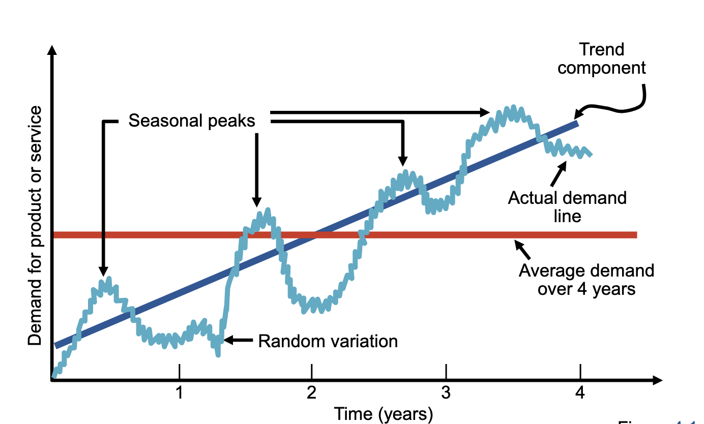
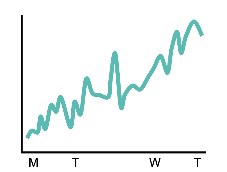
Trend component

Persistent, overall upward or downward pattern

• Changes due to population, technology, age, culture, etc.

• Typically several years in duration

Seasonal component

Regular pattern of up and down fluctuations

• Due to weather, customs, etc.

• Occurs within a single year

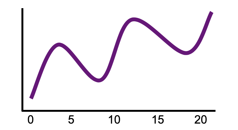
Cyclical component

Repeating up and down movements

• Affected by business cycle, political, and economic factors

• Multiple years in duration

• Often causal or associative relationships

Random component

Erratic, unsystematic, ‘residual’ fluctuations

• Due to random variation or unforeseen events

• Short duration and nonrepeating

Naive approach

Assumes that demand in the next period is equal to demand in the most recent period

• Sometimes cost effective and efficient

• Can be a good starting point

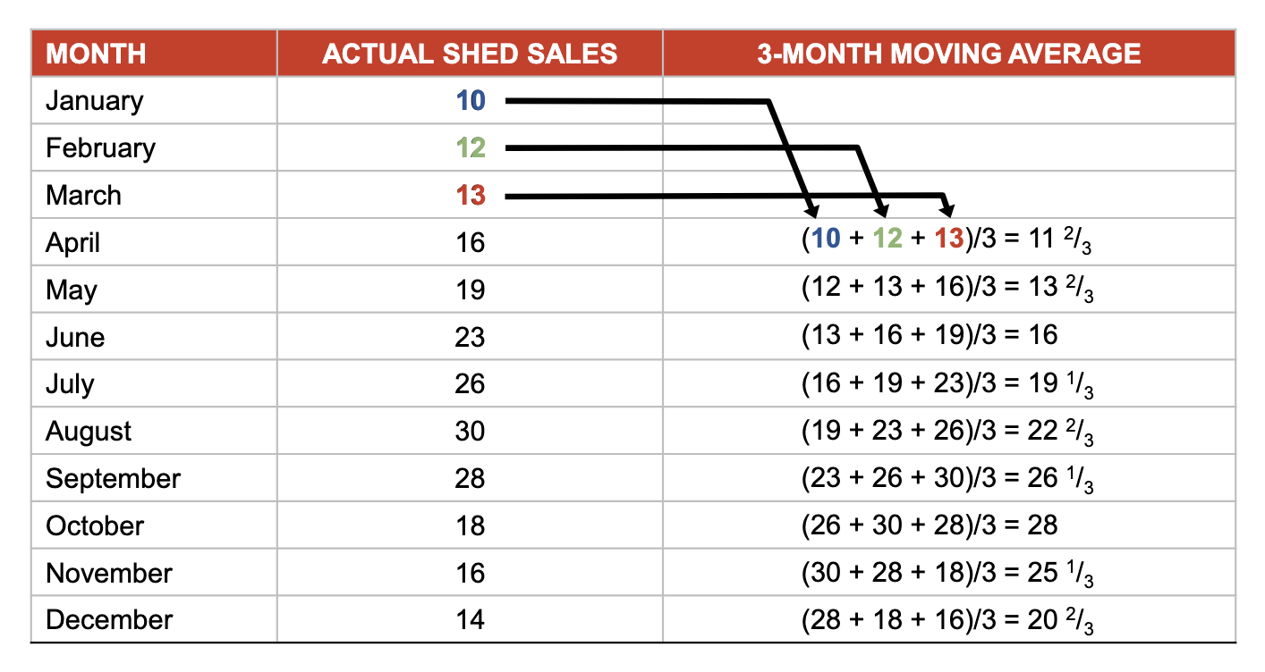
Moving average

Uses an average of the n most recent periods of data to forecast the next period

• A series of arithmetic means

• Used if little or no trend

• Often used for smoothing—provides overall impression of data over time

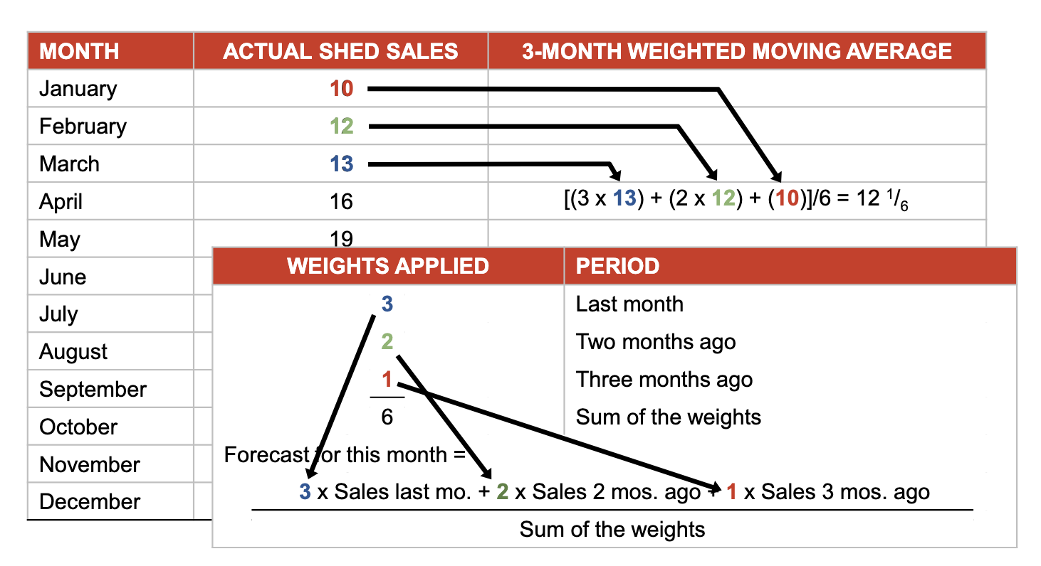
Weighted moving average

Used when some trend might be present with weights based on experience and intuition

• Older data usually less important

Potential problems with moving average

1. Increasing n smooths the forecast but makes it less sensitive to changes

2. Does not forecast trends well

3. Requires extensive historical data

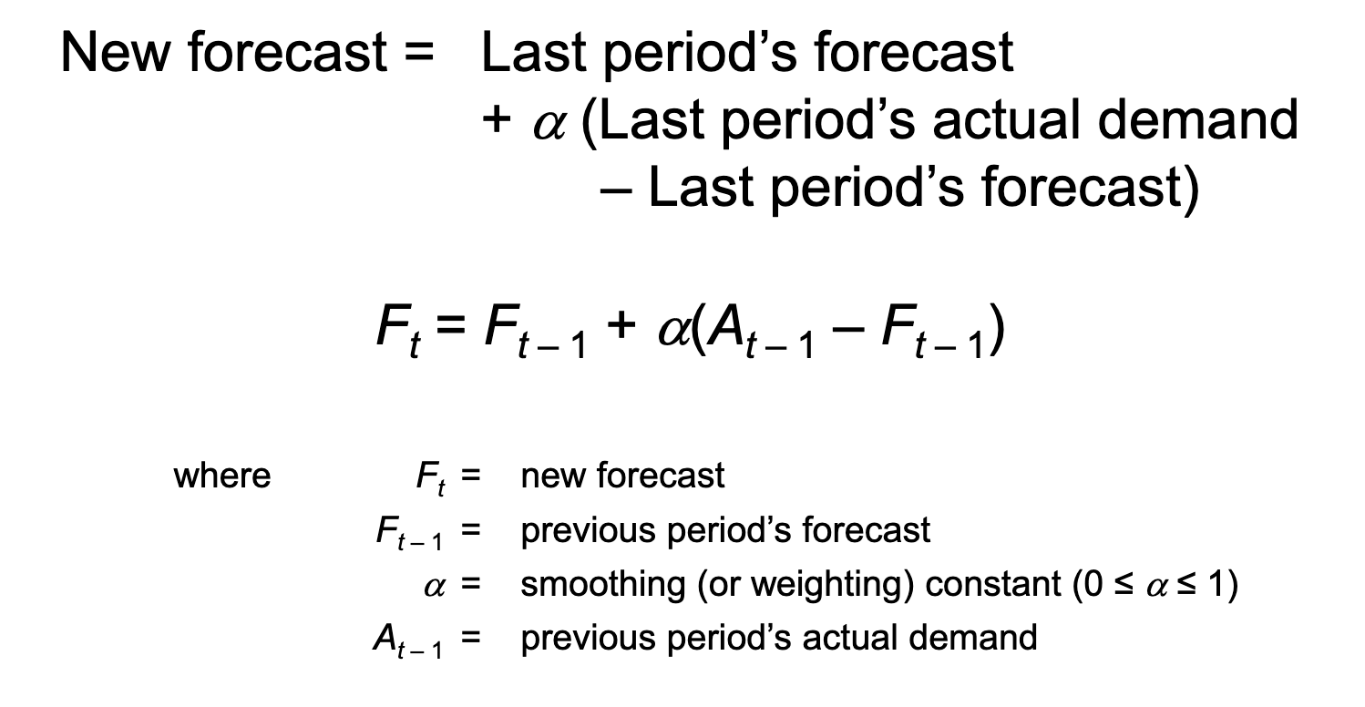
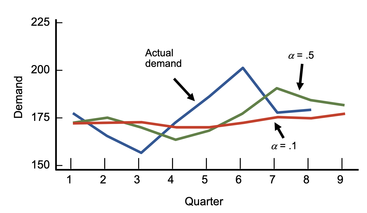
Exponential smoothing

Form of weighted moving average in which data points are weighted by an exponential function

• Weighted decline exponentially

• Most recent data weighted most

• Involves little record keeping of past data

Requires smoothing constant alpha (α)

• Ranges from 0 to 1

• Subjectively chosen (given)

Effect of smoothing constraints

• Smoothing constant generally .05

• As α increases, older values become less significant
  

• Choose high values of α when underlying average is likely to change

• Choose low values of α when underlying average is stable

Selecting the smoothing constant

The objective is to obtain the most accurate forecast no matter the technique

Do this by selecting the model that gives us the lowest forecast error according to one of three preferred measures:

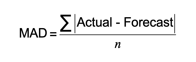
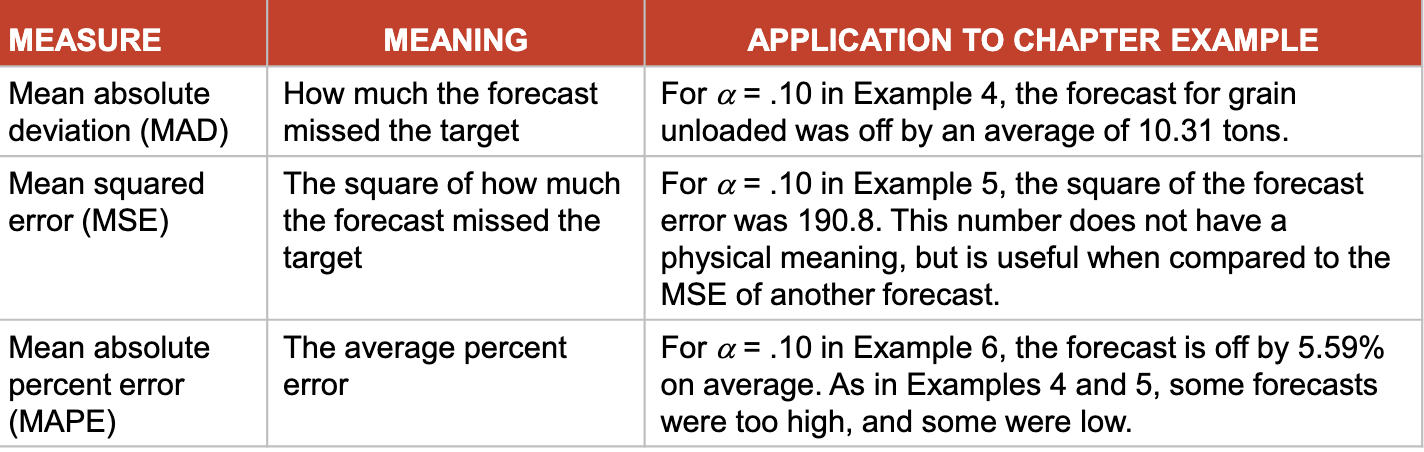
• Mean Absolute Deviation (MAD)

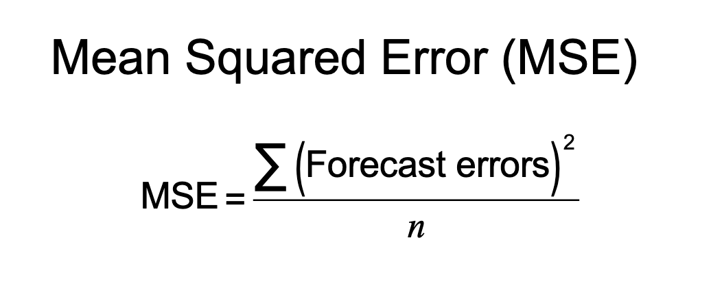
• Mean Squared Error (MSE)

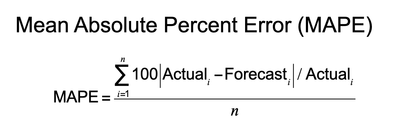
• Mean Absolute Percent Error (MAPE)

Mean Absolute Deviation (MAD)

Computed by taking the sum of the absolute values of the individual forecast errors (deviations) and dividing by the number of periods of data (n)

Mean Squared Error (MSE)

The average of the squared differences between the forecast and observed values

Mean Absolute Percent of Error (MAPE)

Computed as the average of the absolute difference between the forecasted and actual values, expressed as a percentage of the actual values

• Avoids the issue of the magnitude of items forecasted making MAD and MSE disproportionately large

Comparing measures of forecast error

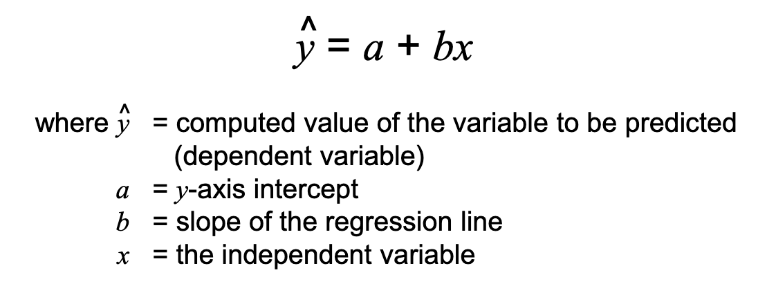
Trend projections

Fitting a trend line to historical data points to project into the medium to long-range

Linear trends can be found using the least squares technique

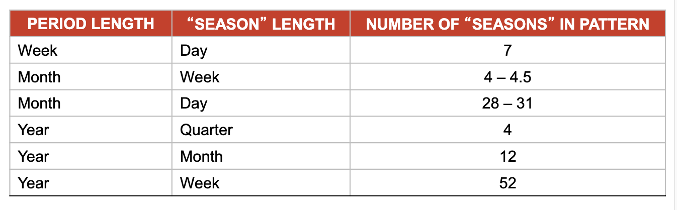
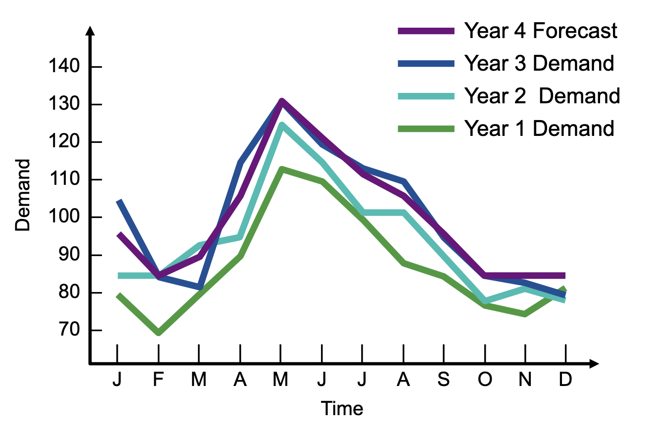
Seasonal variations

Regular upward or downward movements in a time series that tie to recurring events

Can be applied to hourly, daily, weekly, monthly, or other recurring patterns

Calculating seasonal forecasts for monthly seasons

1. Find average historical demand for each month

2. Compute the average demand over all months

3. Compute a seasonal index for each month

4. Estimate next year’s total demand

5. Divide this estimate of total demand by the number of months, then multiply it by the seasonal index for that month

Cycles

Similar to seasonal variations in data but occur every several years (not weeks, months, or quarters)