MT2 Microeconomics

The Production Decisions of a Firm (term and key steps)

The production decisions of firms are analogous to the purchasing decisions of consumers, and can likewise be understood in three steps:

1. Production Technology

2. Cost Constraints

3. Input Choices

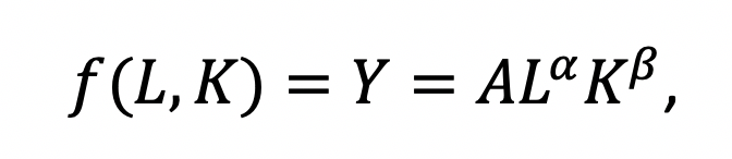
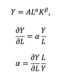
The Cobb-Douglas Production function (term and formula)

Represents the relationship between two or more inputs - typically physical capital and labour - and the number of outputs that can be produced by those inputs

Short run vs long run diff

Short run (capital is fixed; labour is variable) and long run input (both are variables) 

Average (AP) and marginal product (MP) formulas

 AP=QL

Q=TP

MPl=QL=Q2-Q1L2-L1

Incr labour and incr quantity 

MPl=dQdL

Eq,l=QLLQ=MPl1APl=MPlAPl

Average product of labour 

Law of diminishing marginal returns

principle that as the use of an input increases with other inputs fixed, the resulting additions to output will eventually decrease. 

Technology is constant; but if we have an improvement - it

Three stages of a production with one variable input

1. APl=MPl; stage of increasing returns to the factor of production (pos) MPl>0;MPk<0

   1. MP incr and then decr 

   2. AP incr throughout this stage

   3. TP incr sharply 

2. APl=max stage of diminishing returns (diminishing)

   1. MR decr, each additional variable input will still produce add units, but at a decr rate. 

   2. AP starts to diminish 

   3. MP cont to diminish but still posit 

   4. TP incr at diminishing rate till max 

3. MPl=0 stage of negative returns (neg) MOl<0 neg; MPk>0

   1. MR start to become neg - more new inputs - counterproductive , more labour - lessen overall production 

   2. TP curve goes down 

   3. AP curve cont to decr 

   4. MP becomes neg 

Labour productivity

average product of labor for an entire industry or for the economy as a whole

Stock of capital

Total amount of capital available for use in production

Isoquant + map

defines that different combination of inputs (L,K) that produce the same level of input. 

Look like an indifference curve. Isoquant - production in the long-run : L=var; K=var

Short run: L=var; K=fixed (one of them should be fixed) - increasing in dinimishng rate 

Slope for isoquant: negative; convex; cannot intersect; if its far from the origin, it has more level of output ( its better to have more) MRS=MUx/MYy; =delta y/delta x (always 1)

Isoquant map – graph combining a number of isoquants, used to describe a production function.

Isocost

defines the different combination of inputs (L,K) where cost is the same. 

● Slope of Isocost = Slope of Isoquant =-w/r 

Kapital and Labour examples

Kapital - physical (equipment, machineries, facilities)

Labour - workers / working hours

Cost optimisation input rule

The cost optimisation input rule suggests that, optimal combinations of factors of production should be at the point where: 

 Slope of isocost = slope of isoquant

Fixed production function

production function with L-shaped isoquats, so that only one combination of labour and capital can be used to produce each level of output. It describes situations in which methods of production are limited. 

Returns to scale

rate at which output increases as inputs are increased proportionately.

Returns to scale (эффект масштаба) — это то, как изменяется выпуск (output), если ты пропорционально увеличиваешь все факторы производства (капитал, труд и т.д.).

Increasing returns to scale

situation in which output more than doubles when all inputs are doubled.

Constant returns to scale

Situation in which output doubles when all inputs are doubled.

Decreasing returns to scale

Situation in which output less than doubles when all inputs are doubled.

Product transformation curve

Curve showing the various combinations of two different outputs (products) that can be produced with a given set of inputs.

Economies of scope

Situation in which joint output of a single firm is greater than output that could be achieved by two different firms when each produces a single product.

Diseconomies of scope

Situation in which joint output of a single firm is less than could be achieved by separate firms when each produces a single product.

The marginal rate of transformation (MRT)

is the rate at which one good must be sacrificed in order to produce a single extra unit (or marginal unit) of another good, assuming that both goods require the same scarce inputs.

Degree of economies of scope (SC)

Percentage of cost savings resulting when two or more products are produced jointly rather than Individually.

Economic Cost versus Accounting Cost

• Accounting cost - Actual expenses plus depreciation charges for capital equipment.

• Economic cost - Cost to a firm of utilizing economic resources in production, including opportunity cost.

• Opportunity Cost - cost associated with opportunities that are forgone when a firm’s resources are not put to their best alternative use.

• Sunk cost - Expenditure that has been made and cannot be recovered.

• Accounting costs = only explicit costs (actual payments like wages, rent, materials).

• Economic costs = explicit costs + implicit costs, where implicit costs include the opportunity cost of using the firm’s own resources (for example, the owner’s time, owned capital, or foregone rent).

Fixed cost (FC)

Cost that does not vary with the level of output and that can be eliminated only by shutting down.

Average fixed costs – always decline as output increases.

Variable cost (VC)

Cost that varies as output varies.

Marginal cost (MC)

Increase in cost resulting from the production of one extra unit of

output.

Amortization

Policy of treating a one-time expenditure as an annual cost spread out over some number of years.
Amortisation (амортизация) — это постепенное распределение стоимости актива во времени.

Проще: если компания покупает что-то дорогое (например, оборудование), она не списывает всю стоимость сразу, а делит её на части и учитывает как расход в течение нескольких лет.

MP (term)

the additional output created by employing one extra unit of a specific input (like labor or capital), while keeping all other inputs constant. 

Average product (AP)

is a key economics metric measuring the average output produced per unit of variable input (typically labor)

Isocost line

Graph showing all possible combinations of labor and capital that can be purchased for a given total cost. Slope is w/r = MRTS

Expansion path

Curve passing through points of tangency between a firm’s isocost lines and its isoquants.

Cost curves: long vs short run

● long-run average cost curve (LAC) Curve relating average cost of production to output

when all inputs, including capital, are variable.

● short-run average cost curve (SAC) Curve relating average cost of production to output when level of capital is fixed.

● long-run marginal cost curve (LMC) Curve showing the change in long-run total cost as output is increased incrementally by 1 unit.

Diseconomies of scale

Situation in which a doubling of output requires more than doubling of cost. 

Economies of scale

Situation in which output can be doubled for less than a doubling of cost.