ECON 2300 master flash cards

population

complete set of all items that interest an investigator

sample

observed subset, or portion, of a population

sample size denoted as n

parameter

unknown to investigator

numerical measure that describes a specific characteristic of the population

statistic

known to investigator

numerical measure that describes a specific characteristic of the sample.

sampling errors

random differences between sample and population

- cancel out on average

- decrease as sample size grows

nonsampling errors

systematic differences between sample and population

- do not necessarily cancel out on average

- do not necessarily decrease as sample size grows

Margin of error

Margin of error notes

p hat = proportion of sample studied

range of p hat ± ME

only captures sampling error

non response bias

a form of nonsampling error

basically the bias occurring when certain population is more/less likely to respond to survey

summary statistics

summaries of data found. will not be completely accurate

frequency

number of times that a variable takes a certain value in a sample

relative frequency

proportion of times that a variable takes a certain value in a sample

histogram

plot of (relative) frequency by values

some notes on histograms

bins can change size - sometimes necessary to be smaller, bigger, unequal sizing

very important in general

histogram R code

hist(data_name, breaks = (# of bins), xlab = ’x axis label’)

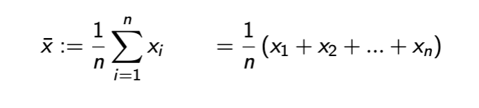
Sample mean

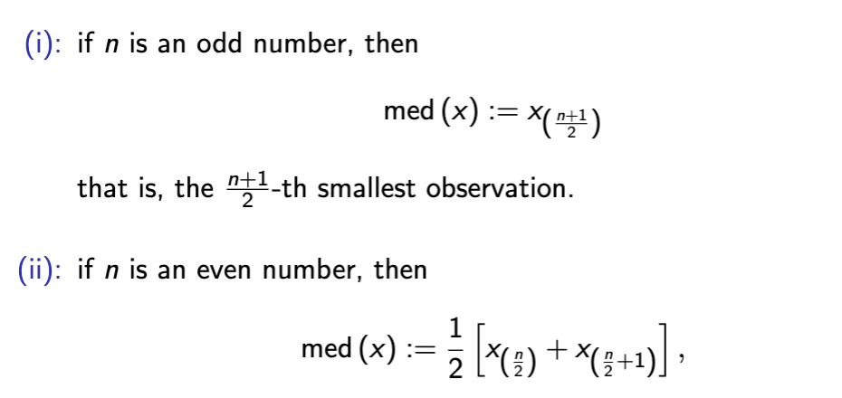
sample median

a cutoff value that is weakly larger than 50% of the sample

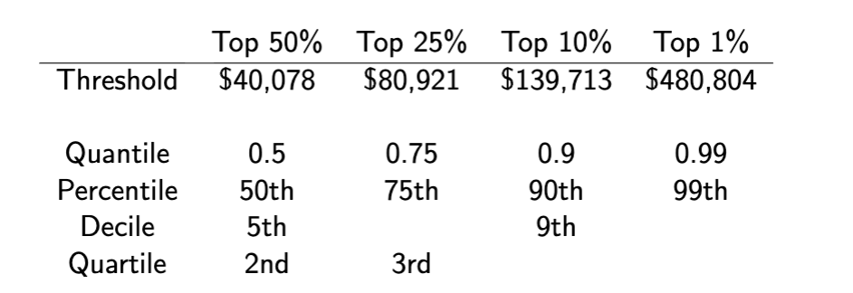
quantile

measure of proportions of data

take any number α between 0 and 1.

− α-quantile = cutoff value that is weakly larger than (100α) % of the sample.

− e.g. median is the 0.5-quantile.

quantile practice

range

maximum observation - minimum observation

less used, we usually use intervals

range R code

range(handspan)

interquartile range

3rd quartile - 1st quartile

less sensitive to outliers

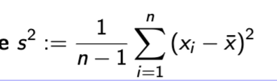
Variance

essentially the average squared difference from the mean.

− division by n − 1 instead of n

− also sensitive to outliers.

Variance R code

var(data_name)

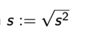
standard deviation

same information as variance

− but more commonly used, since it has the same unit as the data

standard deviation R code

sd(data_name)

basic R commands

table

hist

mean

median

quantile

range

IQR

boxplot

var

sd

access a variable in R

use $ symbol → data_set$var_name

eg to find amount of affairs in affairs file, df_aff$affairs

R cross tabulate 2 tables

table command!

table(data_set$var_one, data_set$var_two)

table(df_aff$affairs, df_aff$gender)

scatterplot in R code

two variables, use plot function

→ variables: disp (displacement), mpg (miles per gallon)

plot(mtcars$disp, mtcars$mpg)

covariance

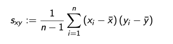
covariance and linear dependence

Zero ⇒ no linear dependence

▶ Positive ⇒ positive linear dependence

▶ Negative ⇒ negative linear dependence

covariance units

product of two variables analyzed

correlation coefficient

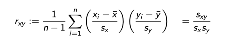
correlation coefficient notes

Centers and standardizes each observation

▶ Bounded between -1 and 1 (later in the course).

correlation and linear dependence

Zero ⇒ no linear dependence

▶ Positive ⇒ positive linear dependence

▶ Negative ⇒ negative linear dependence

if we want to correlate between more than 2 variables

we run a regression

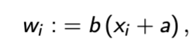
linear transformation of sample x_i

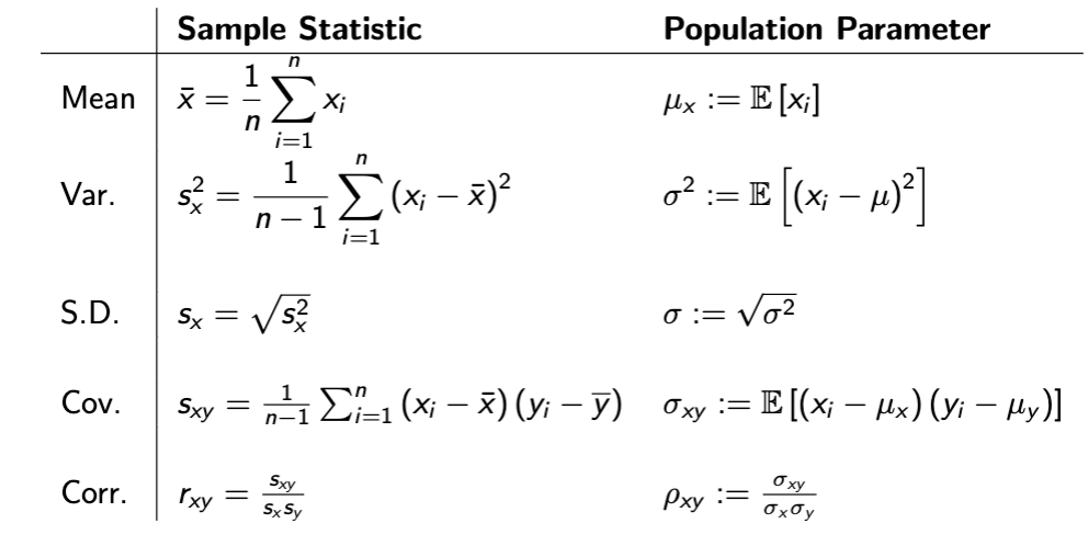
sample stat vs population parameter table

Expectation

form of population mean

can be replaced w/ pictured formula if looking at whole population

law of large numbers

often times, as sample size increases, the sample statistic approximates the corresponding population parameter better and better.

→ the most important result in the foundation of statistics

central limit theorem

often times, when sample size is sufficiently large, the difference between the sample statistic and the corresponding population parameter approximately follows the normal (Gaussian) distribution.

→ the second most important result in the foundation of statistics

R code after lecture 3

var

sd

read.csv

$

attach

table(x,y)

boxplot(x~y)

plot(x,y)

cov(x,y)

cor(x,y)

random experiment

an experiment whose outcomes are random

basic outcome

the finest-grained, relevant outcome of a random experiment

• relevant: depends on what you care about in your random experiment.

• finest-grained: finest categorized, cannot be further divided in a relevant way.

sample space

set of all possible basic outcomes of a random experiment

event

a subset of the sample space.

⇔ equivalently, a set of basic outcomes in the sample space.

Event format

Captial E, e.g. E₁, E₂

E₁ = {HH, HT } - event 1 is heads flipped first

Realization

Only one event in sample space Ω will be realized
signified as ωrealized ∈ E

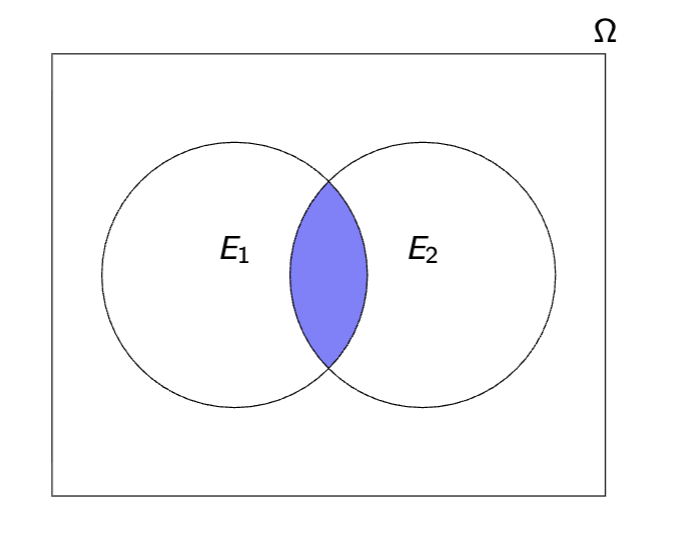
Union E1 ∪ E2

the event that at least one of E1 and E2 occur (if not both)

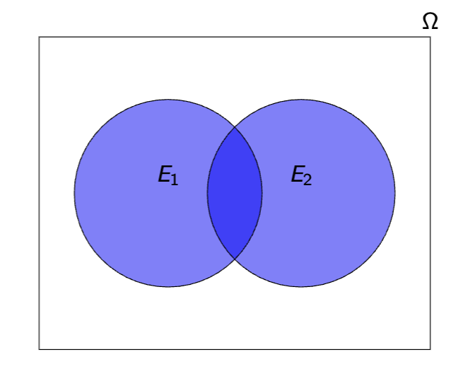
Intersection of Events: E1 ∩ E2

the event that both E1 and E2 occur

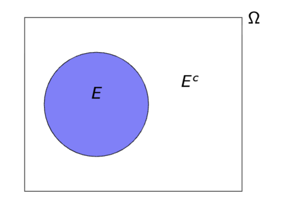
Complement of Event: E^c

Event in which E does not occur

E c ≡ Ω\E := {ω ∈ Ω : ω /∈ E }

Probability P represents

A function of events

In sample space, probability function assigns a number P(E) to E to represent the probability of the event

Axiom 1

0 ≤ P (E ) ≤ 1 for Any Event E

Basically any event must be between 0 and 1

Axiom 2

P (Ω) = 1

The sample space Ω is also a subset of itself

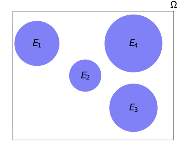
Axiom 3 background: mutual exclusivity

2 Events: mutually exclusive if intersection is empty

E1 ∩ E2 = ∅.

Sequence of events: mutually exclusive in same way

Ei ∩ Ej = ∅, for any i unequal j.

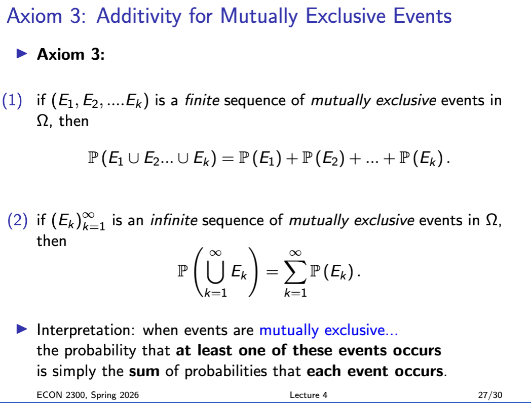
Axiom 3

If E1…En is a set of mutually exclusive events, then probability of several events occurring is just the sum of their probabilities

Classical probability

defined for random experiments in which all basic outcomes are (thought to be) equally likely

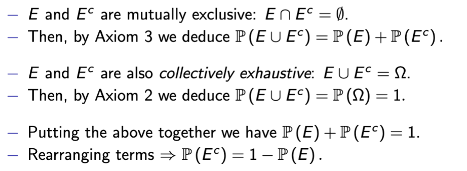
Complement/Logical Negation Rule

P(E^c) = 1 − P(E)

Complement/logical negation proof

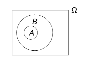
Inclusion/Logical Implication Rule

If event A is included in B and logically implies Event B, then A is less than or equal to B

inclusion symbol A ⊆ B

Events A and B are logically equivalent if

not only A logically implies B,

but also B logically implies A:

then P(A) = P(B)

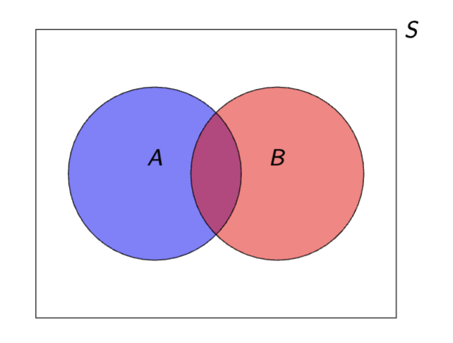
Union/Logical Addition Rule

P (A ∪ B) = P (A) + P (B) − P (A ∩ B) .

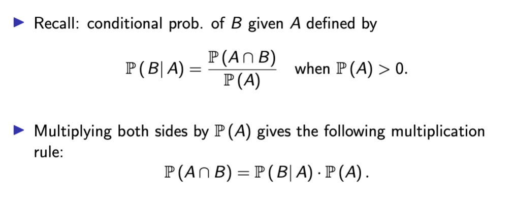
Conditional Probability

If B logically implies the sample space (aka is less than or equal to it) the probability of B given A, or P (B| A) is

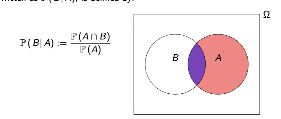
intuition on conditional probability

in conditional probability we set A as the sample space and no longer care about anything outside of it

Conditional Probability Axioms

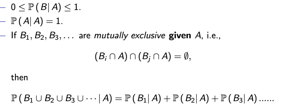
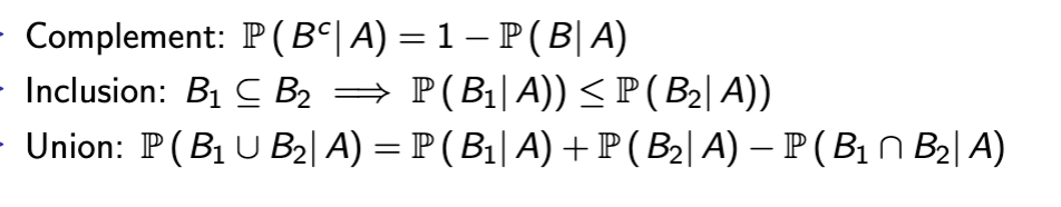
Conditional Probability Rules

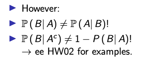
Exceptions on conditional probability rules

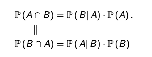
Multiplication Rule Conditional Probability

Multiply both sides of equation by denominator probability to rearrange

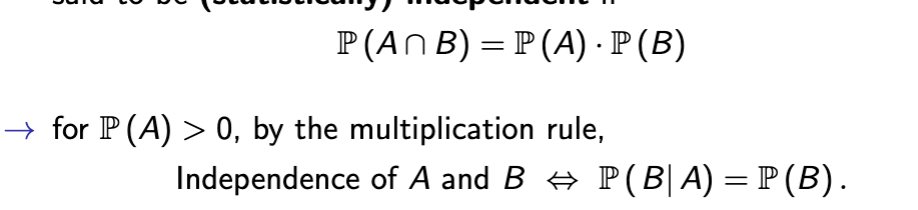
statistical independence

Probability of intersection of events equals the product of both events multiplied, and conditional probability is the probability of the first event in parenthesis

basically shows one event occurs independently of the other

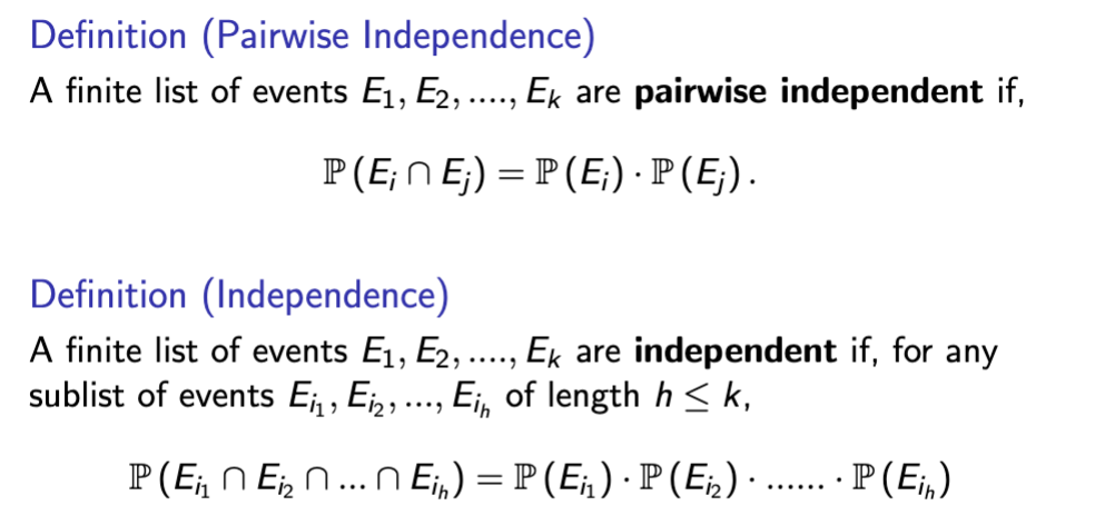
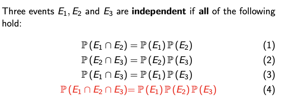
pairwise vs mutual independence

Pairwise independence means any two events in a collection are independent, while mutual (or collective) independence requires that all events are independent jointly

mutual independence implies pairwise dependence among all items in the group, but not vice versa.

mutual independence example

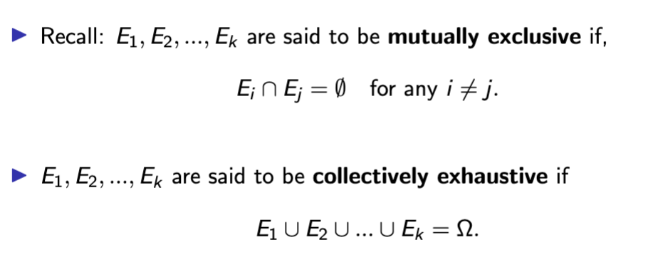
Law of total probability background - mutually exclusive and collectively exhaustive

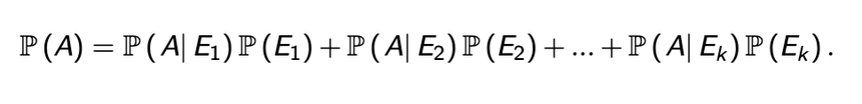
Law of total probability

If a sequence of events E1…n is mutually exclusive and collectively exhaustive, the probability of A is the sum of A conditioned over each event multiplied by that event

Bayes Rule

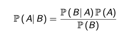
Bayes Rule Proof

then divide both sides by P(B)

Base Rate Fallacy

forgetting about the base rate when forming beliefs

1% of the population is infected with a virus, test accurately detects it 99.99% of the time - that accuracy is the conditional probability over that 1%

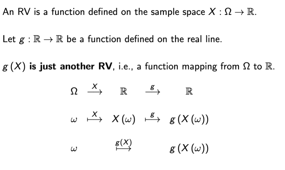
Random Variable

random variables are functions that map out outcomes onto a sample space

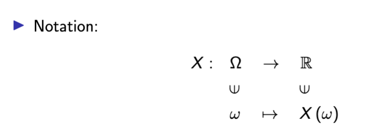
Random Variable Anatomy

RV - function defined on the sample space

Realization - particular numeric value in R that an RV can take on

Format - {X = x} := {ω ∈ Ω : X (ω) = x} ⊆ Ω to represent the probability that Random Variable X takes on x

Support

the set of all possible realizations of a RV.

Supp (X ) := {X (ω) : ω ∈ Ω}

discrete RV

takes on counting numbers, or select values

{0, 1, 2}, {..., −2, −1, 0, 1, 2, ...}, N

Continuous

takes on all values in a segment

support is continuous,

− e.g. [0, 1], (0, ∞), R.

Mixed

support neither discrete nor continuous

− e.g. {−2, −1} ∪ [0, 1]

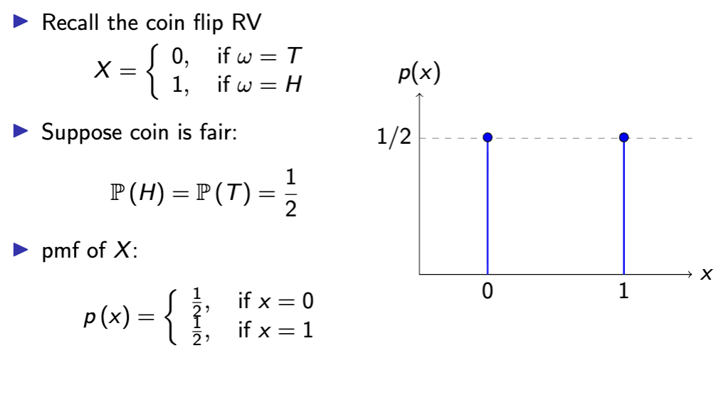
Probability Mass Function

A function of a discrete random variable mapping support of X to real line

Plug in realization x to get probability p(x)

support - p : Supp (X ) → R+

real line - R+ := [0, ∞)

pmf - p (x) := P (X = x)

pmf formatting

function = probability if x takes on value x

When writing pmf x

writing down support is also necessary

The pmf is only (explicitly) defined on the support.

▶ Implicitly: outside the support set, all probabilities are zero.

▶ e.g. for the coin flip RV, Supp (X ) = {0, 1}, and you may write:

p (100) = P (X = 100) = 0.

properties of probability mass functions

between 0 and 1

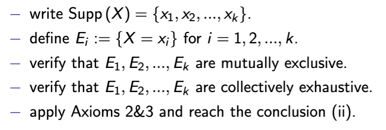
sum of all probabilities over support is 1

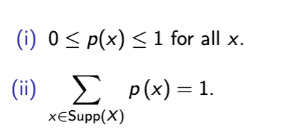
proof of ii pmf rule

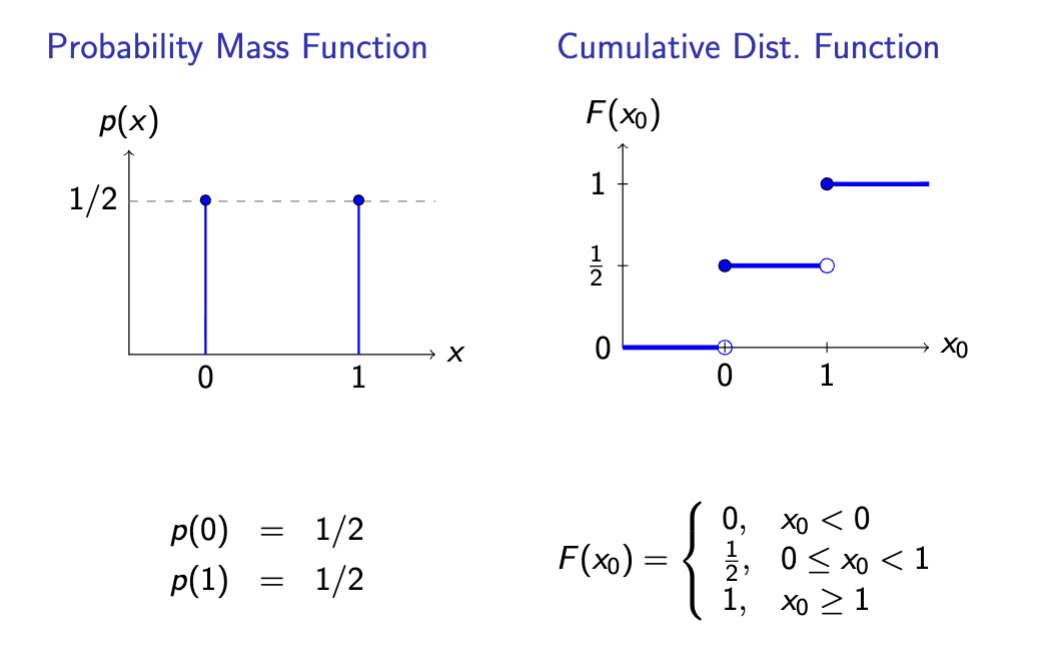
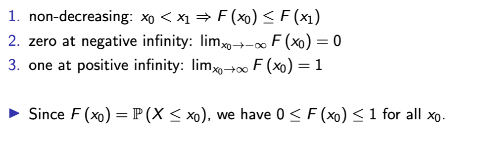
cumulative distribution function

Function of a random variable X representing the cumulative probability of each event - eg probability of X or anything less than it occurring

space F : R → R+

function F (x0) := P (X ≤ x0) , for any x0 ∈ R.

Note: here x0 is not required to be inside Supp (X ).

cdf vs pmf graphs

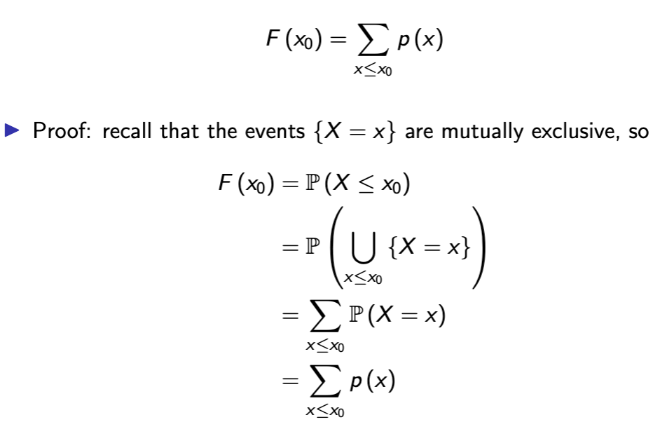
cdf properties

in discrete variables, you can obtain the CDF from the pmf by

adding the pmf

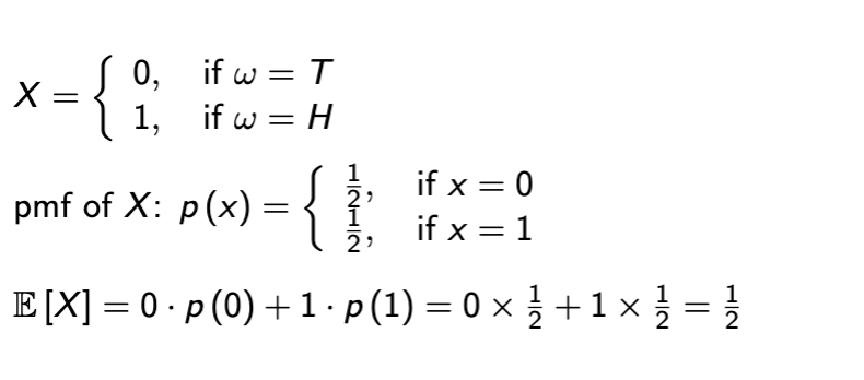
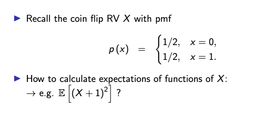
Expectation

mathematical expectation is like a weighted average of a random variable

also written as μ or μx

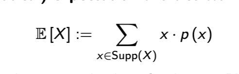
weak expectation from pmf

Function of an RV is

Another RV

more on expectation of a pmf

1. from the example in the screenshot, you can turn the expectation into a function g(x)

2. Plug in each value of X into g(X) - this finds new support of Supp {1, 4}

3. Solve and then multiply each value by respective probability

4. Add to get expectation!

General Formula for Functions of RV

X can be a discrete RV

Y = g(X)

• this means support of Y is {g(X₁), g(X₂),….}

• Here we can have several support values be the same thing

pmf of Y shown in screenshot - basically in english we take the new support of Y and multiply by respective probabilities

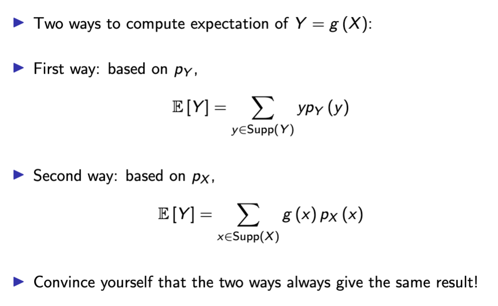
2 ways to compute expectation of a function of an RV

1. Based on the PMF of Y, where you find the PMF first and then multiply by each probability

2. By using the Law of the Unconscious Statistician, in which you calculate g(X) at each point and then find probability

In general

E [g (X )]̸ = g (E [X ])

Expectation of a function doesn’t equal the function of an expectation UNLESS g(X) is linear

linearity of expectation/common expectation transformations

E [aX + b] = a · E [X ] + b