A-Level Economics Theme 1 Flashcards

ceteris paribus

Holding all other things constant to isolate the effects of a variable

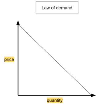
law of demand

When the price of goods/services decreases, the quantity demanded increases and vice versa

marginal utility

The addition satisfaction / benefit the consumer gains after consuming one more unit of a good

Reason economists consider multiple variables when deciding something

So be able to analyse multiple parts of a market at the same time without leaving any parts of it out

behavioural economics

The impact of psychological, social, and emotional factors on economic decisions

normative statement

A statement based on opinion or emotion

positive statement

A provable, factual statement about the world

Fairness

where the society value equality (redistribute income)

opportunity cost

The cost of not choosing the next best alternative

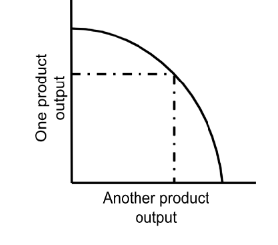
Production probability frontier (PPF)

a graph that illustrates the maximum output of goods/services that the economy can produce, based on the available resources and technology

points inside the PPF 

inefficient

reasons for PPF shift

Due to availability of resources, advancements in technology or improvements in productivity

factors causing PPF to shift outwards

• An increase in natural resources

• Technological advancements

• Human capital development (better education/skill in workers)

• Investment in capital (e.g. infrastructure, machine technology)

• Better management of factor input

• Increase in stock of capital and labour supply

factors causing PPF to shift inwards

• Financial decrease in the consumer or producer

• Lost interest in product

• Price increase in necessary resources

opportunity cost from PPF equation

PPF = Output of factor gained / Output of factor lost

gradient of the PPF

Steep PPF - sacrificing a lot of one product for only a little extra of another product

assumptions of the PPF

• Fixed resources

• A given level of technology

• Full resource utilisation

PPF graph

division of labour

When the production process is broken down into many separate tasks

advantages of division of labour

• Workers become more skilled and proficient in the task and efficiency increases

• Decrease in costs due to increase in quantities

disadvantages of division of labour

• Risk of repetitive strain injury

• Reduced job satisfaction

• Lack of variety in mass produced goods

• Workers take less pride in work - quality suffers

worker turnover

When workers leave jobs and get replaced

functions of money

• Storage of value

• Medium of exchange

• Unit of account

• Standard of deferred payment

characteristics of money

• Hard to counterfeit

• Durable and portable

• Divisible

• Accepted

• Valuable

digital money

Money solely in electronic or digital form

forms of digital money

• Digital wallet

• Cryptocurrencies

• Central Bank digital currencies

• Prepaid cards

reasons for the growth of digital money

• Convenience

• Globalisation

• Security

• Covid-19 pandemic

free market economy

Prices are determined by supply and demand from sellers and buyers

advantages of a free market

• Efficient use of resources

• Wide variety of goods

• Flexibility in price and outputs

disadvantages of a free market

• Inequality in wealth

• Missing markets

• Externalities

command economy

An economy controlled by the government

Advantages of command economies

• Equity goals

• Stability

• Large projects

Disadvantages of command economies

• Inefficiency

• Lack of incentives

• Bureaucracy and corruption

mixed economy

A combination of markets with state intervention in policies

role of the state in a mixed economy

• Public goods provision

• Managing externalities

• Social welfare

• Regulation

• Stabilisation

Rational decision making

One (economic agents, consumers and firms) chooses in a consistent and goal-oriented way

Utility

satisfaction or happiness of a consumer from buying/consuming goods and services

Consumer aims to maximise utility

assumes that when faced with a limited income (budget), a consumer will pick the bundle of goods that gives the highest possible utility

Firms aim to maximise profits

Assumes firm will produce quantity where it makes the largest possible difference between revenue and cost

Marginal revenue

extra revenue from selling one more unit

Marginal cost

extra cost of producing one more unit

Marginal utility

the additional satisfaction or happiness of a consumer buying an extra unit of a good or service

Marginal utility formula

Total utility = marginal utility / profit

Consumer equilibrium assumptions

based on assumption that the income of a consumer is constant and that he spends his entire income on purchasing two goods whose prices are given

Budget line

graphical representation of various combinations of two goods that a consumer can afford at specified prices of the products at particular income level

MC-MR graph MC<MR

each additional unit produced, revenue will be higher than the cost so that you will generate more

MC-MR graph MC>MR

each additional unit produced, the cost will be higher than revenue so that you will create less

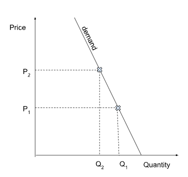
Movement along the demand curve

determined by the change in price of the good itself

Shift of the demand curve

when something other than the price changes

• Right - more demand at every price

• Left - less demand at every price

Conditions of demand curve shift

Income of consumers can change

Income of consumer on demand curve shift

• If average income rises - more people can afford the good or service, therefore the demand curve shifts right

• If the average income falls (recession) - people cut back on luxuries or treats, therefore demand shifts left

Prices of related goods on demand curve shift

• Substitutes (alternatives) - if prices of alternative goods or services become cheaper, therefore demand shifts left

• Complements (bundles) - if price of complementary goods decrease, people buy more of the complementary goods and also the good or service, therefore demand shifts right

Diminishing marginal utility

Every extra unit gives less pleasure than the one before

Point of safety (MR-MC graph)

marginal utility reaches the x-axis, after that point it is dissatisfaction for the consumer

Elasticity of demand

measure the quantity demand of a good or service changes when something else changes (the rate at which demand changes)

Price elasticity of demand (PED) formula

PED = % change in quantity demanded / % change in price

= ΔD (%) / ΔP (%)

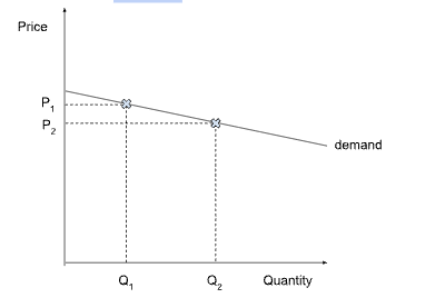
Elastic demand on PED graph

PED > 1 - quantity changes more than price changes

inelastic demand on PED graph

PED < 1 - quantity changes less than the price changes

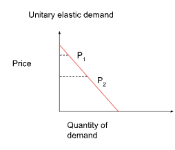
unitary inelastic on PED graph

PED = 1 - quantity and price change at the same rate

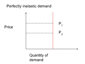
perfectly inelastic on PED graph

PED = 0 - quantity does not change at all when price changes

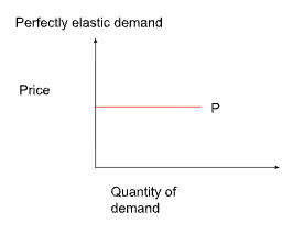
Perfectly elastic on PED graph

PED = ∞ - consumers will only buy at one price and none at any other price

Income elasticity of demand (YED)

how much quantity demanded changes when consumers disposable incomes changes

Income elasticity of demand (YED) formula

YED = % change in quantity demanded / % change in disposable income

= ΔQ demanded (%) / ΔIncome (%)

income elastic on YED graph

YED > 1 - demand rises faster than income (luxury goods)

income inelastic on YED graph

0 < YED < 1 - demand rises but slower than income (Normal necessities)

zero on YED graph

YED < 0 - demand falls when income rises (Inferior goods)

Cross elasticity of demand (XED)

how much a quantity demanded of Good A changes when the price of good B changes

Cross elasticity of demand formula

XED = (%) change in quantity of Good A / (%) change in price of Good B

= ΔQgood 1 (%)/ ΔPgood 2 (%)

XED positive on XED graph

XED > 0 - goods move in the same direction - substitute goods

XED negative on XED graph

XED < 0 - goods move in opposite directions - complementary goods

XED zero on XED graph

XED = 0 - no relationship - unrelated goods

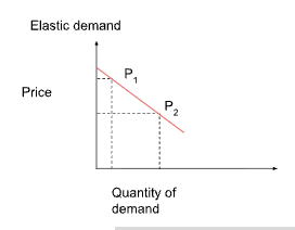
Elastic demand

when change in quantity demanded is relatively larger than price change

Conditions for elastic demand

• Many substitutes available

• Relatively flat demand curve

• Elasticity coefficient is greater than 1

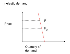
Inelastic demand

when change in quantity demanded is relatively smaller than price change

Conditions for inelastic demand

• Few or no substitutes available

• Relatively steep demand curve

• Elasticity coefficient is less than 1

Factors that make demand more or less elastic:

• availability of substitutes

• Proportion of income

• Time period

• Luxury vs necessity

• Brand loyalty and habit

Reasons firms and governments intervene

• Indirect taxes

• Subsidies

• Real income changes

• Price changes of related goods

Price elasticity and total revenue relationship

Total revenue = Price x Quantity sold

TR = PxQ

Effect of price cut when demand is elastic

increases quantity enough that TR rises

Effect of price cut when demand is inelastic

price cut makes TR fall (you lose more per unit than you gain in extra sales)

Supply

how much of a good or service producers are willing and able to sell at different prices

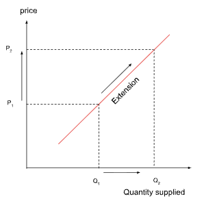
Movement along the supply curve

If market price of the product changes, producers adjust the quantity they supply and you slide up or down the same curve.

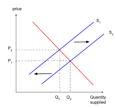
Shifts of the the supply curve

• Sometimes a factor other than the products own price changes, like production costs or technology, and the entire supply curve moves from left or right

• Rightwards shift (S₁ → S₂) - producers are willing to supply more at every price 

• Leftwards shift (S₂ → S₁) - producers less at every price

Key factors for shift in supply

• Increase or decrease Input costs

• New Technologies

• Taxes and subsidies

• Number of suppliers

• Expectations about future prices

• Natural factors and weather

Law of supply

the price of a good or service increases, the quantity supplied will also increase, and vice versa

Price elasticity of supply (PES)

measures the quantity a firm is willing and able to sell changes when price changes.

Price elasticity of supply (PES) formula

PES = %change in quantity supplied / % change in price

PES =∆Q / ∆P

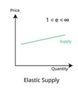
supply relatively elastic on PES graph

PES > 1 - suppliers can increase output more proportionally when price rises

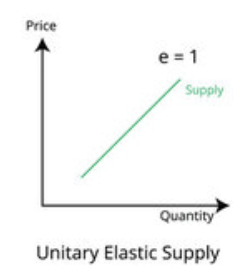
supply unitary elastic on PES graph

PES = 1 - output changes exactly in line with the price

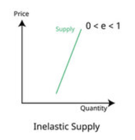
Supply relatively inelastic on PES graph

0 < PES < 1 - the output changes less than price

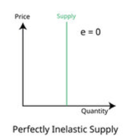
Perfectly inelastic supply on PES graph

PES = 0 - quantity stays the same no matter the price

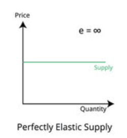
Perfectly elastic supply on PES graph

PES = ∞ - a tiny increase leads to an infinite jump in quantity supplied

• a theoretical construct but it might approximate a scenario where producers can switch instantly and there is a more favourable product in a different market.

Key factors that influence Price elasticity of supply (PES)

• Time period

• Spare capacity

• Mobility of factors

• Stock levels

• Production speed

Short run (short term) response to PES

• At least one factor of production is fixed (eg. capital such as factories and machinery)

• Firms can only vary raw materials or labour

• Supply curve steeper

Long run (long term) response to PES

• All factors are variable - firms can build new factories, adopt new technology or exit the industry

• Supply curve flatter

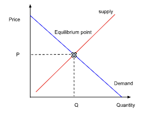
Market equilibrium

a situation in which the quantity of a good or service supplied by producers equals the quantity demanded by the consumers

• State where forces of supply and demand are in balance, leading to stability in prices and quantities exchanged in the market

• Where the Supply curve intersects (how much suppliers are willing to supply at different prices) with the demand curve (how much consumers are willing to buy at different prices)

• The point at which these two curves intersect is known as the equilibrium point and it signifies the price and quantity at which the market clears

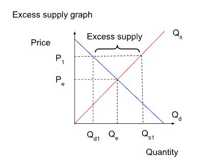
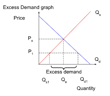
Disequilibrium

prices where demand and supply are out of balance

• Causes a surplus in supply or surplus in demand (or deficit)

Excess supply graph

Excess demand graph

Outward shift in the demand-supply graph

expansion in supply

• Outward shift in demand 

• Increased willingness and ability to buy

• Market can now sustain a higher price

• This higher prices is an incentive for firms to expand production

• Supply responses if there is spare capacity (i.e. s[are factor resources)