Econ Exam #3

the law of demand and price elasticity

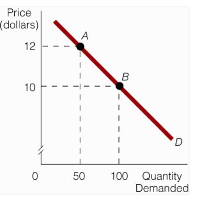
• The law of demand states that price and quantity demanded are inversely related, ceteris paribus 

• But it doesn't tell us by what % the quantity demanded changes as price changes  

• Suppose price rises by 10%. As a result, quantity demanded falls. 

elasticity

The general concept of elasticity provides a technique for estimating the response of one variable to changes in another. It has numerous applications in economics.

Price Elasticity of Demand (Consumers) 

A measure of the responsiveness of quantity demanded to changes in price.  

elasticity is not slope

• for a linear demand function (straight line) slope is constant

• elasticity (Ed) changes along the demand curve

calculating price elasticity of demand

• identify two points on a demand curve

• when calculating price elasticity of demand, we use the average of the two quantities demanded

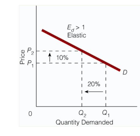
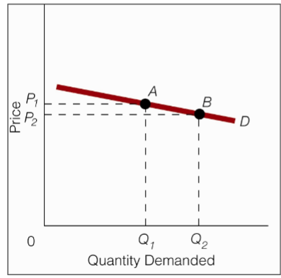
graphical representation of price elastic demand

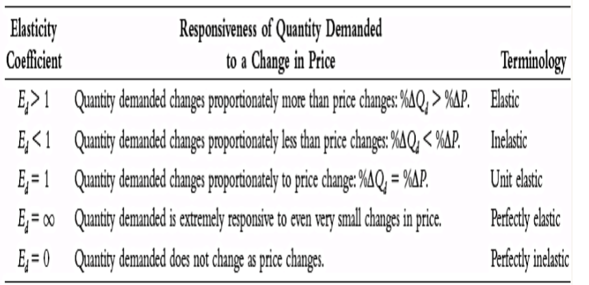
• the % change in quantity demanded is greater than the % change in price

• quantity demanded changes proportionately more than price changes

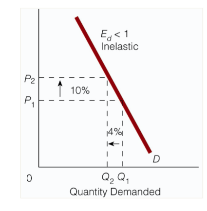
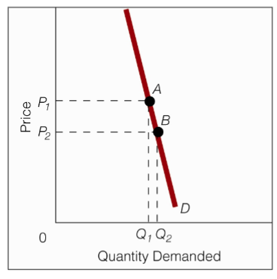
graphical representation of price inelastic demand

• the % change in quantity demanded is less than the % change in price

• quantity demanded changes proportionately less than price changes

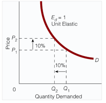
graphical representation of price unitary elastic demand

• the % change in quantity demanded is equal to the % change in price

• quantity demanded changes proportionately to price changes

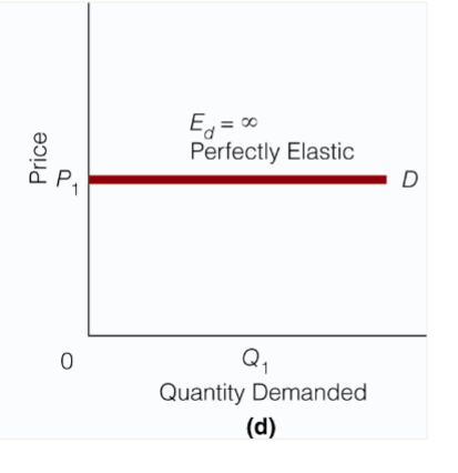
graphical representation of perfectly elastic demand

a small % change in price causes an extremely large % change in quantity demanded (from buying all to buying nothing)

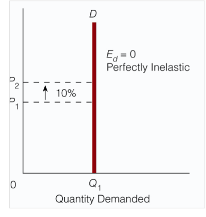
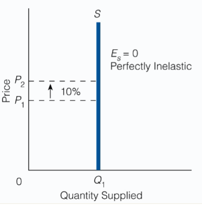
graphical representation of perfectly price inelastic demand

quantity demanded doesn’t change as price changes

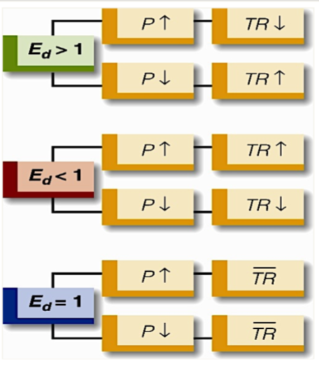
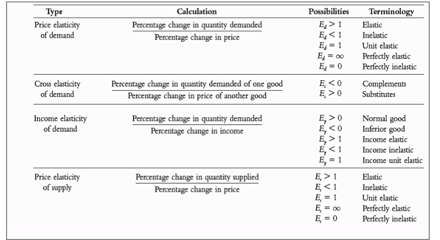
price elasticity of demand summary

price elasticity and total revenue

total revenue (TR): of seller equals the price of a good times the quantity of the good sold (PxQ)

elastic demand and total revenue

• if demand is elastic, the % change in quantity demanded is greater than the % change in price

• when demand is elastic, price and total revenue are inversely related

inelastic demand and total revenue

• if demand is inelastic, the % change in quantity demanded is less than the % change in price

• when demand is inelastic, price and total revenue are directly related

unit elastic demand and total revenue

if demand is unit elastic, the % change in quantity demanded is equal to the % change in price

elasticity, price changes, and total revenue

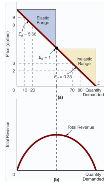
price elasticity of demand along a straight-line demand curve

• In (a), the price elasticity of demand varies along the straight-line downward-sloping demand curve.

• There is an elastic range to the curve (where Ed > 1) and an inelastic range (where Ed < 1).

• At the midpoint of any straight-line downward-sloping demand curve, price elasticity of demand is equal to 1 (Ed = 1)

• Part (b) shows that in the elastic range of the demand curve, total revenue rises as price is lowered. I

• In the inelastic range of the demand curve, further price declines result in declining total revenue.

• Total revenue reaches its peak when price elasticity of demand equals 1.

detriments of price elasticity

• # of substitutes

• necessities versus luxuries

• % of ones budget spent on the good

• time

number of substitutes

the more substitutes for a good, the higher the price elasticity of demand; fewer substitutes for a good, the lower the price elasticity of demand

necessities versus luxuries

generally, the more that a good is considered a luxury (a good that we can do without) rather than a necessity (a good that we can’t do without), the higher the price elasticity of demand

% of ones budget spent on the good

the greater the % of one’s budget that goes to purchase a good, the higher the price elasticity of demand; the smaller the % of one’s budget that goes to purchase a good, the lower the price elasticity of demand

time

the more time that passes (since the price change), the higher the price elasticity of demand for the good; the less time that passes, the lower the price elasticity of demand for the good

cross elasticity of demand

measures the responsiveness in quantity demanded for one good to changes in the price of another

• ex: hot dogs and ketchup/mustard are complements

• ex: hot gods and burgers are substitutes

income elasticity of demand

measures the responsiveness of quantity demanded to changes in income

• income elastic: the % change in quantity demanded of a good is greater than the % change in income

• income inelastic: the % change in quantity demanded of a good is less than the % change in income

• income unit elastic: the % change in quantity demanded of a good is equal to the % change in income

price elasticity of supply

measures the responsiveness of quantity supplied to changes in price

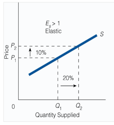
graphical representation of elastic supply

The percentage change in quantity supplied is greater than the percentage change in price: Es > 1 and supply is elastic.

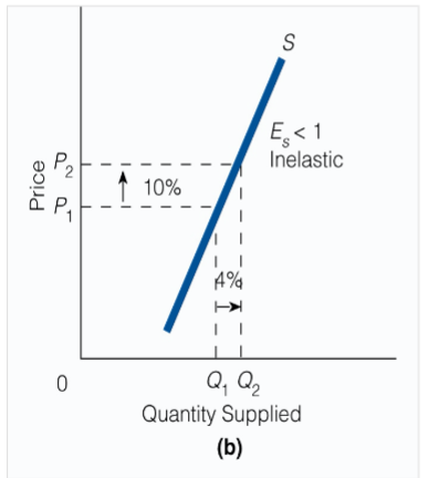
graphical representation of inelastic supply

The percentage change in quantity supplied is less than the percentage change in price: Es < 1 and supply is inelastic.

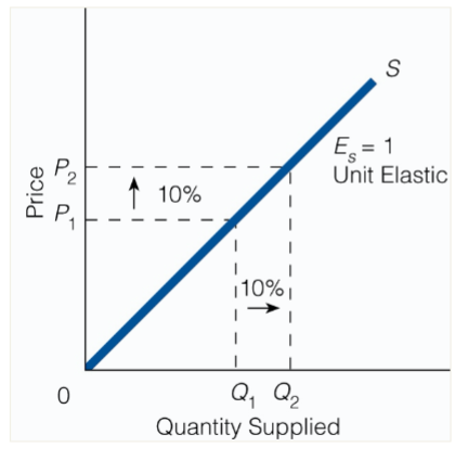
graphical representation of unit elastic supply

The percentage change in quantity supplied is equal to the percentage change in price: Es = 1 and supply is unit elastic.

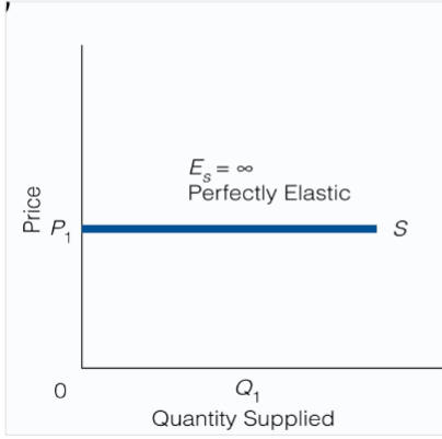
graphical representation of perfectly elastic supply

A small change in price changes quantity supplied by an infinite amount: Es = ∞ and supply is perfectly elastic.

price elastic graphical representation of supply

A change in price does not change quantity supplied: Es = 0 and supply is perfectly inelastic.

price elasticity of supply and time

• The longer the period of adjustment is to a change in price, the higher the price elasticity of supply will be.

• This refers to goods whose quantity supplied can increase with time, a characteristic of most goods. The obvious reason is that additional production takes time.

• It does not, however, cover instances when additional production may be impossible, say, original Picasso paintings.

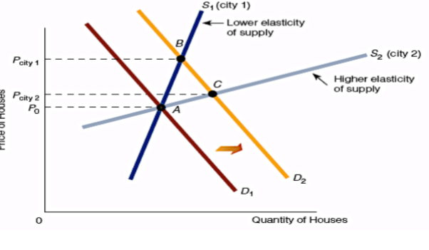
housing prices and elasticity of supply

• S1 rep resents the supply of housing in city 1, and S2 represents the supply of housing in city 2.

• S1 has lower elasticity of supply than S2.

• Suppose the demand for housing in each city rises from D1 to D2. As a result, the price of houses rises in both cities, but it rises by more in city 1 than city 2. In other words, the lower the elasticity of supply, the greater the increase in price.

summary of the four elasticity concepts

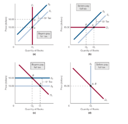
elasticity and the tax

utility theory

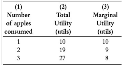
• Utility is a measure of the satisfaction, happiness, or benefit that results from the consumption of a good 

• A UTIL is an artificial construct used to measure utility 

• Total utility is the total satisfaction a person receives from consuming a particular quantity of a good 

• Marginal utility is the additional utility a person receives from consuming an additional unit of a particular good 

law of diminishing marginal utility

• The marginal utility gained by consuming equal successive units of a good will decline as the amount consumed increases 

• The total utility of something can be rising as the  marginal utility of that something is falling 

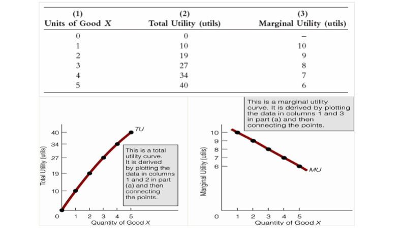
total utility, marginal utility, and the law of diminishing marginal utility

• Both total utility and marginal utility are expressed in utils 

• Marginal utility is the change in total utility divided by the change in the quantity consumed of the good 

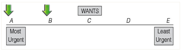
law of diminishing marginal utility- application

• the law of diminishing marginal utility is based on the idea that if a good has a variety of uses but only 1 unit of the good is available, then the consumer will use the first unit to satisfy his or her most urgent want

• if 2 units are available, the consumer will use the second unit to satisfy a less urgent want

interpersonal utility comparison

Comparing the utility of one person receives from a good, service, or activity with the utility another person receives from the same good, service, or activity 

no interpersonal utility comparison

Caution: the utility obtained by one person cannot be scientifically or objectively compared with the utility obtained from the same thing by another person bc utility is subjective 

consumer equilibrium

• The analysis is based on the assumption that individuals seek to maximize utility 

• Occurs when the consumer has spent all income and the marginal utilities per dollar spent on each good purchased are equal 

• Where the letters A-Z represent all the goods a person buys 

marginal utility analysis and the law of demand

• Marginal utility analysis can be used to illustrate the law of demand, which states that price and quantity demanded are inversely related, ceteris paribus. 

• Starting from consumer equilibrium in a world containing only two goods, A and B, a fall in the price of A will cause MUA /PA to be greater than MUB /PB. 

• As a result, the consumer will purchase more of good A to restore herself to equilibrium. 

marginal utility analysis and the law of demand

• Marginal utility analysis can be used to illustrate the law of demand, which states that price and quantity demanded are inversely related, ceteris paribus. 

• Starting from consumer equilibrium in a world containing only two goods, A and B, a fall in the price of A will cause MUA /PA to be greater than MUB /PB. 

• As a result, the consumer will purchase more of good A to restore herself to equilibrium. 

diamond-water paradox

• The paradox: Water is cheap, and diamonds are expensive! 

• The observation that things that have the greatest value in use sometimes have little value in exchange and things that have little value in use sometimes have the greatest value in exchange. 

• How can this be explained??? 

• Utility theory provides a solution! 

diamond-water paradox resolved

• The total utility of water is high because water is extremely useful. 

• The total utility of diamonds is low in comparison because diamonds are not as useful as water. 

• The marginal utility of water is low because water is so plentiful that people end up consuming it at low marginal utility. 

• The marginal utility of diamonds is high because diamonds are so scarce that people end up consuming them at high marginal utility. 

• Do prices reflect total or marginal utility? Marginal utility. 

behavioral economics

• Behavioral economists argue that some human behavior doesn't fit neatly- at a minimum, easily- into the traditional economic framework 

• Behavioral economists believe they have identified human behaviors that are inconsistent with the model of men and women as rational, self-interested, and consistent 

these behaviors include the following

1. Individuals are willing to spend some money to lower the incomes of others even if it means their incomes will be lowered 

2. Individuals don't always treat $1 as $1; some dollars seem to be treated differently from other dollars 

3. Individuals sometimes value a good more if it is theirs than if it isn't theirs and they are seeking to acquire it (endowment effect) 

business firm

• An entity that employs factors of production (resources) to produce goods and services to be sold to consumers, other firms, or the government 

• Supply side 

market coordination- invisible hand

The process in which individuals perform tasks, such as producing certain quantities of goods, based on changes in market forces, such as supply, demand, and price 

managerial coordination and business firms- visible hand

The process in which managers direct employees to perform certain tasks 

why do business firms arise in the first place?

• Firms are formed when benefits can be obtained from individuals working as a team 

• Efficiency of working together 

• Sum of team production > sum of individual production 

problem of and solutions for “team” work

• problem: shirking- the behavior of a worker who is putting forth less than the agreed to effort

  • solution: monitor- person (manager) in a business firm who coordinates team production and reduces shirking

• problem: monitor shirking

  • solution: make the monitor a residual claimants- persons who share the profits of a business firm

• the efficiency wage theory (above-market wage will reduce shirking)

• human resource management

why firms exist as an alternative to having a separate contract with each factor of production- Ronald Coase

• “The costs of negotiating and concluding a separate contract for each exchange transaction which takes place on a market must also be taken into account. . . .

• It is true that contracts are not eliminated when there is a firm, but they are greatly reduced. A factor of production (or the owner thereof) does not have to make a series of contracts as would be necessary, of course, if this co-operation were a direct result of the working of the price mechanism. For this series of contracts is substituted one.

• At this state, it is important to note the character of the contract into which a factor enters that is employed within a firm. The contract is one whereby the factor [the employee], for a certain remuneration (which may be fixed or fluctuating), agrees to obey the directions of an entrepreneur within certain limits.” Ronald Coase

markets: inside and outside the firm

• economics is largely about trades or exchanges; it’s about market transactions

• in supply-and-demand analysis, the exchanges are btw buyers of goods and services and sellers of goods and services

• in the theory of the firm, the exchanges take place at two levels:

  • (1) at the level of individuals coming together to form a team

  • (2) at the level of workers choosing a monitor

• employees submit to the monitor’s commands because they realize that only a well-known team will yield the benefits they desire

firm’s objective: maximizing profit

The difference btw total revenue and total cost 

explicit and implicit cost

• explicit cost- a cost incurred when an actual (monetary) payment is made

• implicit cost- a cost that represents the value of resources used in production for which no actual (monetary) payment is made (opportunity cost)

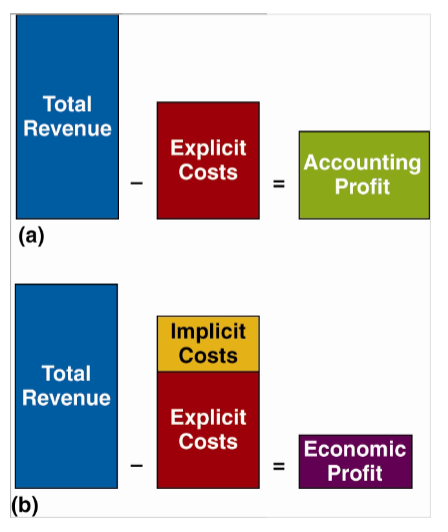
accounting, economic, and normal profit

• Accounting profit: the diff btw total revenue and explicit costs 

• Economic profit: the diff btw total revenue and total cost, including both explicit and implicit costs 

• Normal profit: zero economic profit. A firm that earns normal profit is earning revenue equal to its total cost (explicit plus implicit costs). This is the level of profit necessary to keep resources employed in that particular firm 

production and cost: fixed and variable inputs

• Production is a transformation of resources or inputs into goods and services 

• Fixed input: an input whose quantity cannot be changed as output changes 

• Variable input: an input whose quantity can be changed as output changes 

production and cost: short and long run

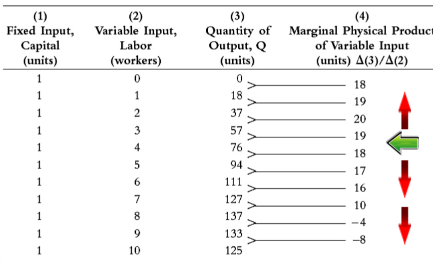
marginal physical product (MPP)

The change in output that results from changing the variable input by one unit, holding all other inputs fixed 

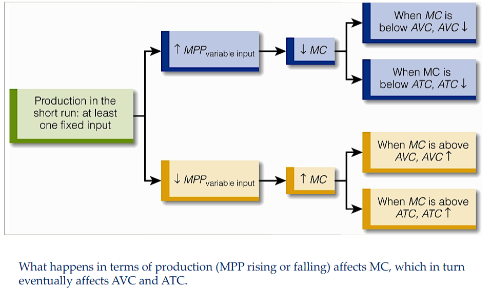
production in the short run and the law of diminishing marginal returns

• In the short run, as additional units of variable input are added to fixed input, the marginal physical product of the variable may increase at first 

• Eventually, the marginal physical product of the variable input decreases 

• The point at which marginal physical product decreases is the point at which diminishing marginal returns have set in 

law of diminishing marginal returns

As ever-larger amounts of a variable input are combined with fixed inputs, eventually, the marginal physical product of the variable input will decline 

production in the short run and the law of diminishing marginal productivity

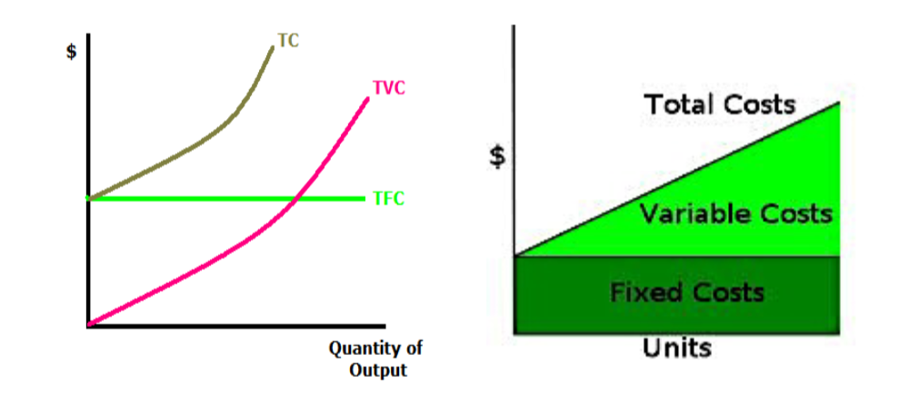
fixed, variable, total, and marginal cost

• Fixed costs (FC): costs that do not vary with output; the costs associated with fixed inputs 

• Variable cost (VC): costs that vary with output; the costs associated with variable inputs 

• Total cost (TC): the sum of fixed costs and variable costs. TC = TFC + TVC 

• Marginal cost (MC): the change in total cost that results from a change in output  

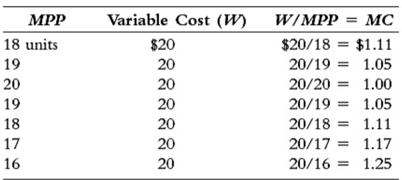
marginal physical product and marginal cost

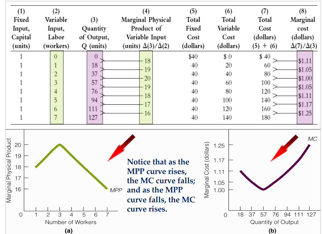
how MPP affects MC

average productivity

• When the news media uses the word productivity, it is usually referring to average physical product instead of marginal physical product 

• To illustrate the difference, suppose 1 worker can produce 10 units of output a day and 2 workers can produce 18 units of output a day.

• Marginal physical product is 8 units (MPP of labor = ∆Q / ∆L). Average physical product, which is output divided by quantity of labor is equal to 9 units.

labor productivity

• Labor productivity is used in newspapers and in gov docs, it refers to the average (physical) productivity of labor on an hourly basis 

• By computing the average productivity of labor for diff countries and noting the annual % changes we can compare labor productivity btw and within countries  

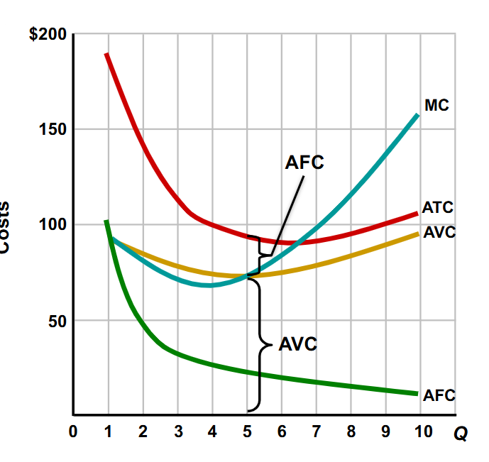
average fixed, variable, and total cost

• Average fixed cost (AFC): total fixed cost divided by quantity of output 

• Average variable cost (AVC): total variable cost divided by quantity of output 

• Average total cost (ATC) or Unit Cost: total cost divided by quantity of output 

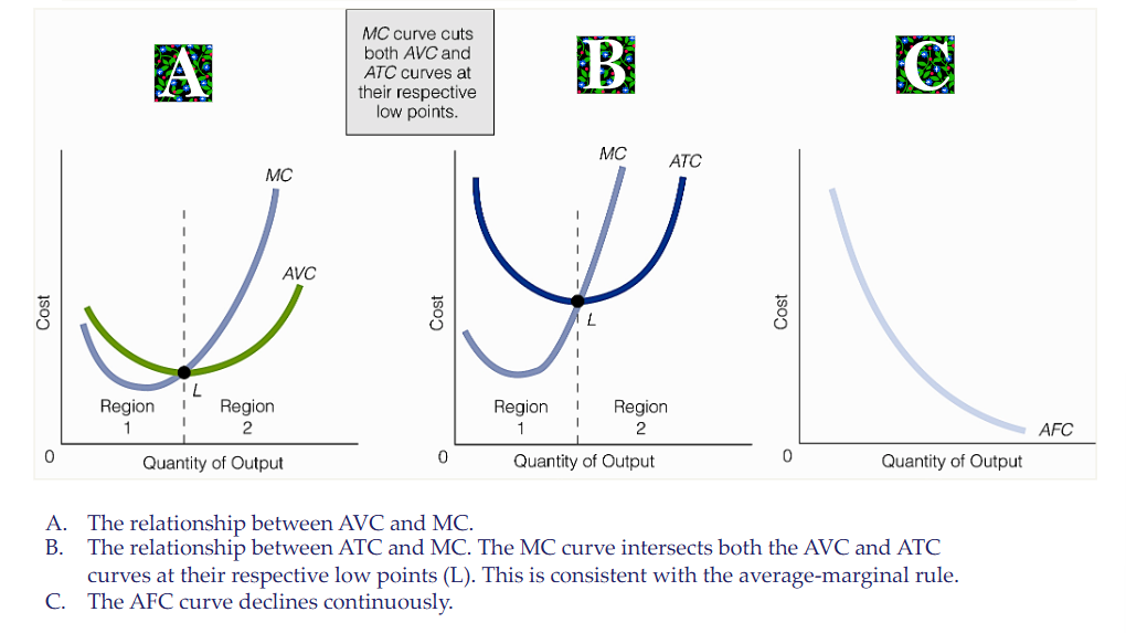
average-marginal rule

• When the marginal magnitude is below the average magnitude, the average magnitude falls 

• When the marginal magnitude is above the average magnitude, the average magnitude rises 

average and marginal cost curves

tying short-run production to costs

sunk cost

• A cost incurred in the past that cannot be changed by current decisions and therefore cannot be recovered 

• Economists advise individuals to ignore sunk costs 

production and costs in the long run

• In the short run, there are fixed costs and variable costs; therefore, total cost is the sum of the two 

• A period of time in which all inputs in the production process can be varied (no inputs are fixed). In the long run, there are no fixed costs, so variable costs are total costs 

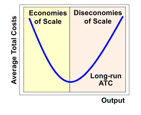
long-run average total cost (LRATC) curve

A curve that shows the lowest (unit) cost at which the firm can produce any given level of output 

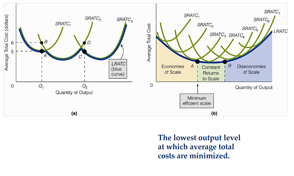
• there are three short-run average total cost curves for three different plant sizes

• if these are the only plant sizes, the long-run average total cost curve is the heavily shaded, blue scalloped curve

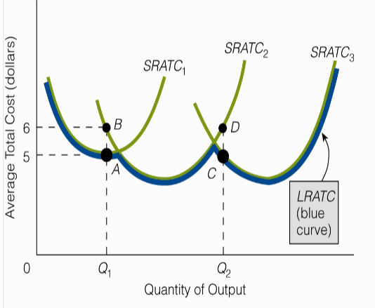
LRATC

• the long-run average total cost curve is the heavily shaded, blue smooth curve

• the LRATC curve is not scalloped because it’s assumed that there are so many plant sizes that the LRATC curve touches each SRATC curve at only one point

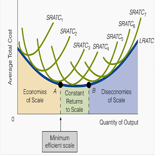
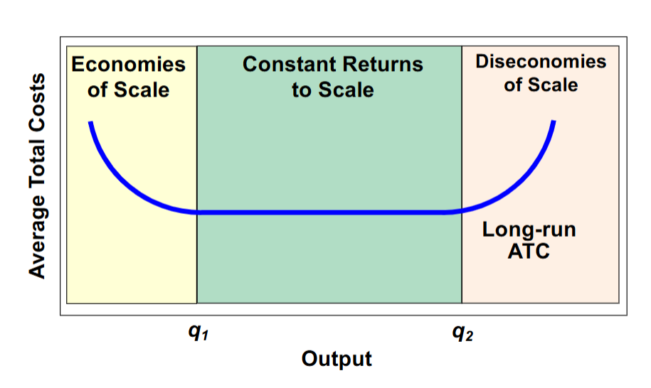
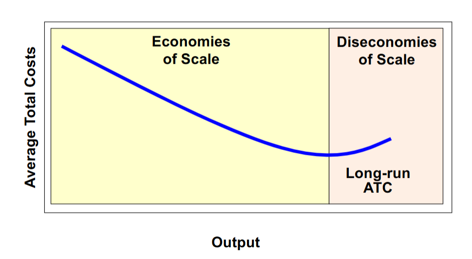
economies of scale

• Economies of Scale exist when inputs are increased by some percentage and output increases by a greater percentage, causing unit costs to fall. (LRATC is falling)

• Constant Returns to Scale exist when inputs are increased by some percentage and output increases by an equal percentage, causing unit costs to remain constant. (LRATC is constant)

• Diseconomies of Scale exist when inputs are increased by some percentage and output increases by a smaller percentage, causing unit costs to rise. (LTRAC is rising)

• Minimum Efficient Scale - The lowest output level at which average total costs are minimized.

why economies of scale?

• Up to a certain point, long-run unit costs of production fall as a firm grows. There are two main reasons for this:

  • Growing firms offer greater opportunities for employees to specialize.

  • Growing firms can take advantage of highly efficient mass production techniques and equipment that ordinarily require large setup costs and thus are economical only if they can be spread over a large number of units.

why diseconomies of scale?

In very large firms, managers often find it difficult to coordinate work activities, communicate their directives to the right persons in satisfactory time, and monitor personnel effectively.

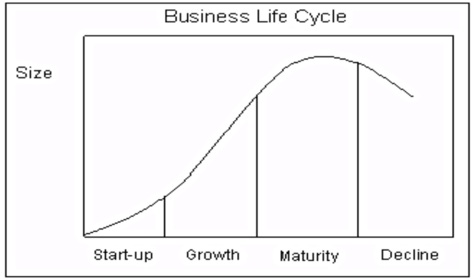
business life cycle

shifts in cost curves

a firm’s cost curves will shift if there is a change in:

• taxes

• input prices

• technology

cost curves

long-run production costs

• the firm can change all input amounts, including plant size

• all costs are variable in the long run

• long-run ATC

  • different short-run ATCs

economies of scale

• economies of scale

  • labor specialization

  • managerial specialization

  • efficient capital

  • other factors

• constant returns to scale

diseconomies of scale

• control and coordination problems

• communication problems

• worker alienation

• shirking

minimum efficient scale (MES)

• lower level of output where long-run average costs are minimized

• can determine the structure of the industry

MES and Industry Structure

TFC, TVC, and TC

market structure

A particular environment of a firm, the characteristics of which influence the firm's pricing and output decisions 

diff forms of market structure

• Perfect competition 

• Monopolies 

• Oligopolies  

the theory of perfect competition

• A theory of market structure based on four assumptions: 

1. There are many sellers and many buyers, none of which is large in relation to total sales or purchases. 

2. Each firm produces and sells a homogeneous product. 

3. Buyers and sellers have all relevant information with respect to prices, product quality, sources of supply, and so on. 

4. There is easy entry into and exit from the industry. 

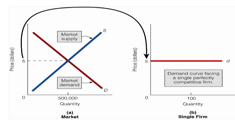
a perfectly competitive firm is a price taker

A seller that doesn't have the ability to control the price of the product it sells; it takes the price determined in the market 

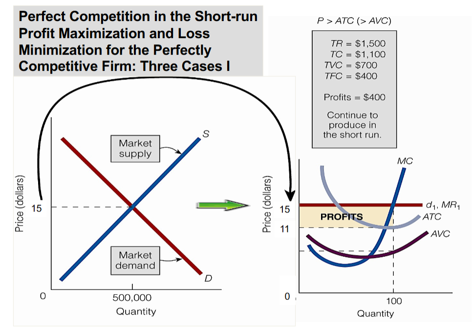
market demand curve and firm demand curve in perfect competition

• The market, composed of all buyers and sellers, establishes the equilibrium price (a) 

• A single perfectly competitive firm then faces a horizontal (flat, perfectly elastic) demand curve 

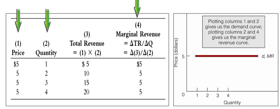
marginal revenue (MR)

The change in total revenue that results from selling one additional unit of output 

the demand curve and the marginal revenue curve for a perfectly competitive firm

• by computing marginal revenue, we find that it is equal to price

• by plotting columns 1 and 2, we obtain the firm’s demand curve

• by plotting columns 2 and 4, we obtain the firm’s marginal revenue curve

• the two curves are the same

quantity of output the perfectly competitive firm will produce

The firm’s demand curve is horizontal at the equilibrium price. Its demand curve is its marginal revenue curve. The firm produces that quantity of output at which MR = MC

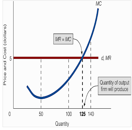
profit maximization rule

• profit is maximized by producing the quantity of output at which MR = MC

• for perfect competition, profit is maximized when P = MR = MC

resource allocative efficiency

• Producing a good—any good—until price equals marginal cost ensures that all units of the good are produced that are of greater value to buyers than the alternative goods that might have been produced.

• A firm that produces the quantity of output at which price equals marginal cost (P = MC) is said to exhibit resource allocative efficiency.

• For a perfectly competitive firm, profit maximization and resource allocative efficiency are not at odds.

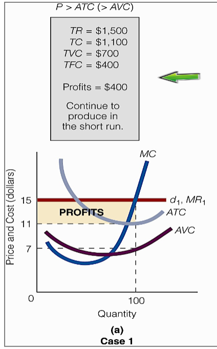
perfect competition in the short-run

• profit maximization and loss minimization for the perfectly competitive firm - case I

• in case 1, TR TC and the firm earns profits

• it continues to produce in the short run

perfect competition in the short-run

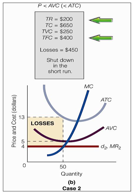
• profit maximization and loss minimization for the perfectly competitive firm - case II

• in case 2, TR < TC and the firm takes a loss

• it shuts down in the short run bc it minimizes its losses by doing so