3.10 Method of Variation of Parameters
1/3
There's no tags or description
Looks like no tags are added yet.
Name | Mastery | Learn | Test | Matching | Spaced | Call with Kai |
|---|
No analytics yet
Send a link to your students to track their progress
4 Terms
The Variation of Parameters
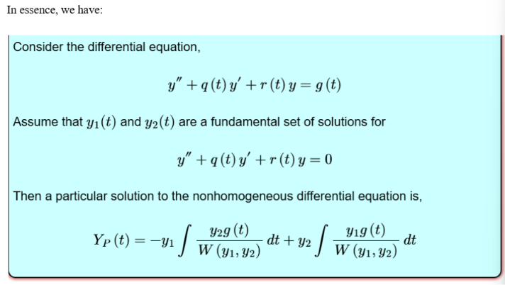
Any non-homogenous 2nd order differential equation can be solved by the application of the variation of parameters method; in essence, we must do the following process when applying this algorithm:
Identify the complementary solution of the homogenous version of the function.
Solve for both u1(x) and u2(x)
Multiply both y1(x) and y2(x) by u1(x) and u2(x) respectively
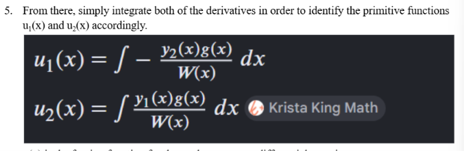
Solving for u1(x) and u2(x)
y1(x), y2(x) → complementary solution sets
g(x) → forcing function
W(x) → Wronskian of both y1(x) and y2(x)
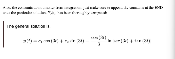
Final Solution
Final Solution Example
Notice how the final solution, y(t), is a combination of both the complementary solution and the product of u1(x) and u2(x).