Intro to NLP (Week 1 & 2)

Symbolic vs Statistical vs Generative/Neural/DL NLP

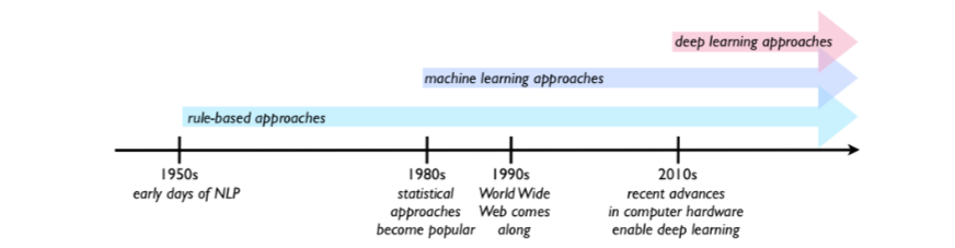
Symbolic(rule-based NLP) (1950-1990) relies on hard coded rules and templates: reliable but unscalable to non stylistic, ambiguous language. Sentiment analysis on symbolic NLP is very weak

• ELIZA (early chatbot)

Statistical NLP leverages statistical info to create probabilistic/generative models that learn distribution over language and generate text. Requires high data availability (HDA) and high quality data.

• WWW benefited the growth of statistical NLP due to HDA

Neural Networks learn representations automatically from raw text and replaces features with (EMBEDDING VECTORS). Sequences are models with RNNs, LSTMs, GRUs (2010-2017) and Transformers(2017)

• learn distributed representations(embeddings) to capture semantic similarity. Scales better with large corpora = better performance. Better at modelling long range dependencies.

• Data hungry and compute intensive and can hallucinate

Early NLP experiment (1950)

Georgetown IBM experiment. russian → english translation which helped launch NLP as a field

Why did early rule-based NLP systems struggle?

Rule-based systems had one major strength: when a case was covered by the rules, they could be reliable because the knowledge came from human experts. But they struggled because language is:

• creative,

• ambiguous,

• constantly changing,

• full of exceptions.

• hard to build a complete and scalable set of rules.

What was the main advantage and main bottleneck of statistical NLP?

The main advantage of statistical NLP is that it does not need rigid hand-crafted assumptions about language in advance. Instead, it can learn patterns from data, which makes it more scalable and flexible than pure rule-based approaches.

The main bottleneck is data: these methods need large amounts of high-quality, representative data. In machine translation, improvements in the 1980s were strongly tied to the availability of large amounts of parallel data, where texts in one language are aligned with equivalent texts in another.

How did the WWW help NLP?

The growth of the World Wide Web made massive amounts of text available, which helped statistical NLP methods improve. In tasks like machine translation, the availability of large parallel corpora was especially important because systems could learn translation relationships from real examples.

Pretraining a model to Fine tuning

GPT (language modelling)

BERT (masked language modelling) (bidirectional context)

After pretraining the general model it needs to be fine tuned

• Classification: Sentiment Analysis

• Sequence Labelling: Named Entity Recognition

• Seq2Seq : Translation

NLP applications

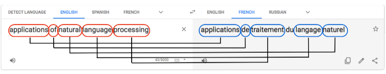
Google Translate (machine translation)

• challenging because different language have different rules/definitions for words different forms of words based on gender and number. Differences in word order also add complexity. Words themselves are ambiguous.

• parallel data contains annotation for the chunks of text on both sides that express precisely the same idea. Learn to identify the correspondences between the two parts at level of granularity

Information Retrieval/Information Search

• How to search and retrieve quickly with millions of documents on the web. How to rank relevance. Queries may be imprecise, incomplete, ungrammatical or ambiguous? Book (for reading or booking hotel?)

Spam Detection (text classification task)

• Challenging since some emails contain clear red flags but some are normal content. The cost of false alarms? Must balance false positives and negatives. Combination of signals instead of one signal feature

• Binary classification approach

Predictive Text

• Challenging as the range of possible responses is practically infinite. Ability to accurately predict bring ML closer to human

• provided with a large number of examples, computers can observe what characters and word combinations are most likely and predict

Linguistic Analysis

• Raw text processing – segmentation and tokenization.

• Morphology – stemming and lemmatization. (sub word level)

• Word level – part-of-speech tagging.

• Syntax – grammatical relations, chunking, parsing.

• Semantics – word meaning and text meaning.

Stemming vs Lemmatisation

Stemming cuts off prefixes and suffixes.

• Downside is the root form may not be a valid word running → run.

• Efficient and scalable

• Stemming can merge dimensions, which can reduce vector space dimensionality (good for computation) > cost of stemming errors

Advantages of stemming:

• it does not rely as heavily on a dictionary,

• it can handle new or creative words better,

• it can reduce dimensionality more aggressively.

A lemma is a dictionary form where we can map multiple forms to the most basic one (Reduces space).

• Lemmatisation is resource intensive and time consuming since algorithm has to keep a dictionary of lemmas to convert word forms.

• Uses look up tables with rule sets.

• Returns more understandable base forms.

• Can be improved with PoS

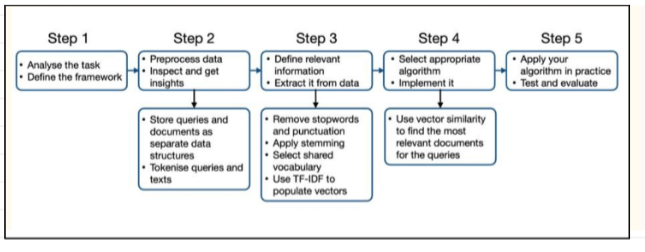
NLP Project Pipeline

Step 1(Analysis): Split the dataset, remove punctuation with regex, convert to lowercase (define the task, inputs/outputs, pick framework (e.g classification problem)

Step 2(data exploration +preprocessing): Lowercasing, tokenisation, stopword removal, punctuation, lemmatisation or stemming. Store queries and docs in clearly defined data structures (e.g dictionaries of queries, collections of documents(

Step 3: Feature engineering, consider weight of features (textual: n-grams, tf-idf, bag of words), normalisation: remove punctuation, lowercase, remove stopwords) . Build a shared vector space, which may have some 0s as words are not present.

Step 4: The model(transformers, LSTM vs logistic regression), naive bayes, apply cosine similarity between the query vector and doc vector

Step 5: Evaluate with accuracy, precision, MRR, baselines and benchmarks.

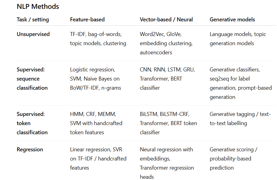
NLP Methods

Symbolic/Feature-based NLP

• Manual linguistic or count-based representations

• “Hand-engineered text representations such as bag-of-words, n-grams, and TF-IDF. Usually sparse and interpretable.”

Statistical / traditional ML NLP

• Learns from feature counts using classical ML

• Naive Bayes, logistic regression, SVM, HMM

Vector-based / neural

• “Represents text numerically as dense vectors (embeddings), either static or contextual, and uses neural networks.”

• Word2Vec, LSTM, BERT, Transformers

Generative models

• “Learn probability distributions over text and can generate new sequences; sometimes also used for classification or labelling.”

• n-gram LM, seq2seq, GPT, T5

In information retrieval, what are a document, collection, term, and query?

In information retrieval (IR), the core objective is to find relevant, usually unstructured, information (such as text, images, or documents) within a large repository to satisfy a specific user need

A document is any unit of text indexed for retrieval.

A collection is the set of documents being searched

. A term is an item, often a word or phrase, used by the system to represent content.

A query is the user’s information need expressed as a set of terms.

Tokenisation

tokenization or word segmentation is the task of separating out (tokenizing)words from running text. Most important step in text processing

Multi-word expressions are phrases like New York Stock Exchange that behave like a single conceptual unit even though they contain spaces. Tokenizing them incorrectly can damage meaning

tokenization systems are designed to be fast and reliable, often using deterministic methods such as regular expressions compiled into finite-state automata, together with lists of abbreviations and machine-learning-based refinements.

Frequency Analysis and Zipfs Law

Frequency analysis studies how often words occur in a corpus. It helps reveal patterns in the data, such as which words are very common and may be uninformative for a task.

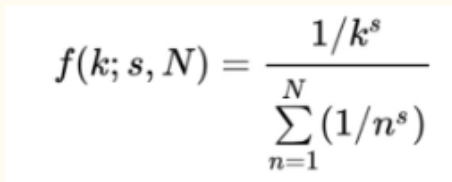
Zipf's Law is an empirical law stating that in a large corpus of natural language, the frequency of any word is inversely proportional to its rank in a frequency table. The Power Law Distribution: If you rank words by frequency, the r -th most frequent word has a frequency proportional to 1/r^α (where α is close to 1)

Normalised frequency of the element of the rank is in the picture: (where s is the exponent of language.) English is s=1

Zipf’s law explains why we see so many very frequent words, many of which become stopwords in tasks like IR or classification. It also explains the long tail of rare terms and why feature selection matters so much.

What are stopwords, and why are they often removed?

Stopwords are very frequent words that carry relatively little meaning on their own in many NLP tasks. Examples are common function words like “the”, “of”, and “and”.

In information retrieval, removing stopwords is useful because:

• they often do not express the core information need,

• they increase the dimensionality of the search space,

• filtering them helps produce a smaller, more informative representation of the query or document.

stopwords are not “useless” in an absolute sense. They can contribute grammatical structure (depends on task)

Vector Representation

In the vector-space model, both queries and documents are represented as vectors in the same space, where dimensions correspond to terms. The values in each dimension often represent counts or weights for those terms.

e.g a query with two terms can be represented as a two-dimensional vector where each coordinate corresponds to how often each term appears.

Similarity between query and document can then be measured geometrically.

Length/ norm and dot product of a vector

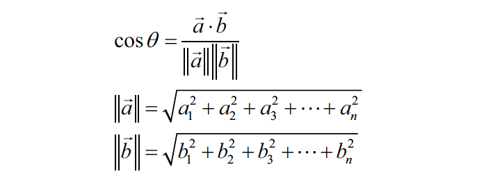
The length (norm) of a vector tells us how large it is. For a vector u = [u1, u2, ..., un], the Euclidean norm is: ||u|| = sqrt(u1^2 + u2^2 + ... + un^2)

This matters because cosine similarity divides by vector lengths to normalise for document/query size.

The dot product measures how much two vectors align. A larger dot product usually means greater similarity, but it is affected by vector length. For vectors u and v, the dot product is: u · v = u1v1 + u2v2 + ... + unvn

This is the key formula behind cosine similarity

Angle between two vectors

The relationship is: u · v = ||u|| ||v|| cos(theta)

Cosine Similarity

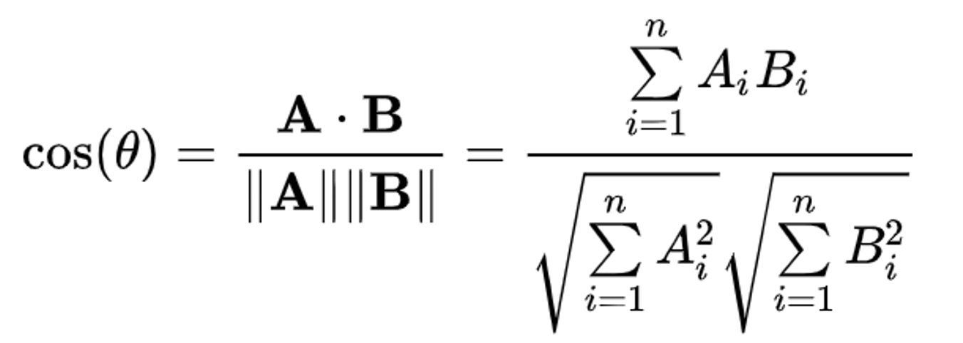
Cosine similarity measures the cosine of the angle between two vectors. The formula is: cosine(A,B) = (A · B) / (||A|| ||B||)

It compares direction rather than raw size, which makes it very useful in IR.

Expanded form in images

Cosine Similarity vs Plain Dot Product

The plain dot product tends to favour longer vectors, so longer documents may look more relevant simply because they contain more words. Cosine similarity fixes this by dividing by the lengths of the vectors, so it focuses on direction / relative term distribution instead of absolute size.

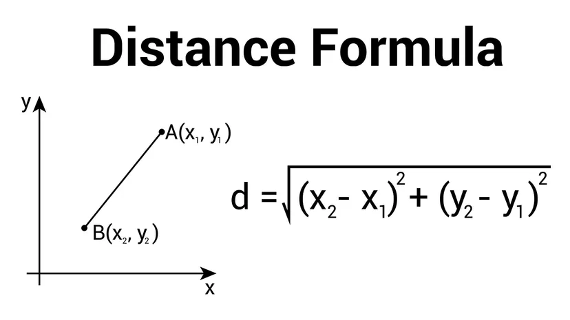
Cosine similarity vs euclidean distance

Euclidean distance is heavily affected by document length, while cosine similarity is length-normalised and focuses on direction.

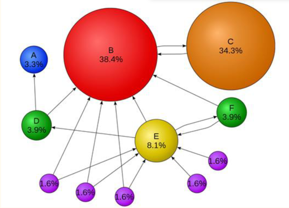
What is PageRank

PageRank is a search-ranking idea that looks not just at the words on a page but also at how pages link to each other. Links from other pages act a bit like endorsements, helping determine which pages are important. A page gets a high PageRank if the random surfer is likely to visit it often

This models the idea that a user usually follows links, but sometimes jumps to a random page.

PageRank algorithm

Step 1: Start with initial PageRank values

If there are 4 pages, a simple start is to give each one the same value:

PR(A) = PR(B) = PR(C) = PR(D) = 0.25

Step 2: For each page, look at incoming links. Find which pages point to that page.

Step 3: Compute contribution from each incoming page
If page v links to u, then its contribution is:

PR(v) / L(v)

Step 4: Add all contributions. That gives the new PageRank of page u.

• PR(u) = PageRank of page u

• B_u = set of pages that link into page u

• PR(v) = PageRank of page v

• L(v) = number of outgoing links from page v

• N = number of pages

• d = damping factor

To calculate the PageRank of page u, add up the contribution from every page v that links to u. Each linking page gives: PR(v) / L(v)

PR(u) = sum over v in B_u of PR(v) / L(v)

PR(u) = Σ_{v ∈ B_u} PR(v) / L(v)

The slides note a damping factor often taken as:

d=0.85

• with probability d, the user keeps following links

• with probability 1 - d, the user jumps to a random page

• experimentally, d = 0.85

PR(u) = (1 - d) + d * Σ_{v ∈ B_u} PR(v) / L(v) OR

PR(u) = (1 - d)/N + d * Σ_{v ∈ B_u} PR(v) / L(v)

Step 5: Repeat

Keep recalculating all page scores until the changes become very small.

Repeat until the change is < some ε

That means stop when the change is less than a tiny threshold ε.

TF-IDF

Term frequency (TF) is the idea that the more often a key term appears in a document, the more relevant that document may be to that term.

TF(term)=1term in document​×number of occurrences

Inverse document frequency (IDF) measures how informative or rare a term is across the whole collection.

• if a term appears in many documents, it is less useful for distinguishing relevance,

• if a term appears in few documents, it is more informative.

IDF(term) = log10(N / (DF(term) + 1)) (+1 not always needed)

where:

• N = total number of documents,

• DF(term) = number of documents containing the term.

The +1 smooths the count to avoid division-by-zero problems, and the logarithm tones down very large raw differences

TF-IDF combines local importance and global rarity:

• TF says how important a term is within a document,

• IDF says how distinctive that term is across the collection.

So:

TF-IDF(term) = TF(term) × IDF(term)

This means a term gets a high score when it occurs often in a document and is not common across all documents. TF-IDF scores are then used to build document vectors for search.

Term weighting vs raw counts

Raw counts are helpful, but not all terms are equally informative. IR uses term weighting so that the algorithm focuses more on salient, useful words and less on words that are common everywhere.

Weighting improves efficiency and relevance.

• a term that appears many times in one document may matter,

• but if it appears in almost every document in the collection, it is not very discriminative.

That is why term weighting moves beyond simple counts toward measures like TF, IDF, and TF-IDF.

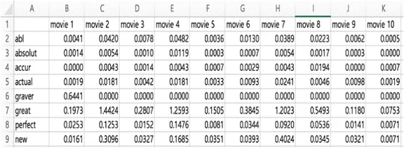
TF Matrix

A TF-IDF matrix is a table that shows the TF-IDF weight of each term in each document.

Usually:

• rows = documents

• columns = terms

• cell value = TF-IDF score of that term in that document

So it is basically a way of turning text into numbers so documents can be compared mathematically.

the TF-IDF matrix is part of the vector space model.

Precision and mean precision

Precision@k measures the proportion of the top k returned documents that are relevant:

P@k=# relevant documents in top k/ k = relevant documents in top k​

It focuses on the top of the ranking, which is what users usually care about most.

Mean P@k = (1 / Q) * sum of (P_i@k) where Q is the total number of queries

It focuses on the top results, which is where users usually pay most attention in search systems.

MRR (Mean reciprocal rank)

Reciprocal rank is based on the position of the first relevant result for one query. MRR is the average reciprocal rank across multiple queries. MRR measures how early the first relevant result appears, which reflects how quickly a user finds a useful answer.

RR = 1 / rank of first relevant result

MRR = (1 / Q) * sum of (1 / rank_i) where Q is the total number of queries and rank_i is the position of the first relevant document for query i

What is a web crawler

A web crawler is a program that recursively downloads web pages to build a searchable index. It is one of the foundations of large-scale web search engines.

What is the difference between directory-style access and search

A directory organises content by a human-defined hierarchy and users browse through categories. A search system lets users issue queries and retrieves documents algorithmically. As the web grew, search became necessary because manual directory-style organisation no longer scaled well.

What is the difference between a forward index and an inverted index? (IR)

A forward index and inverted index are about how a search engine stores and looks up text efficiently.

A forward index stores which words occur in each document.
An inverted index stores, for each word, which documents contain it.
Search engines rely heavily on inverted indexing because it makes query lookup much faster.