Molecular Impact of Variants

How can sequence variants affect GLP-1R function at the molecular level

Sequence variants (amino acid changes) can alter:

• Ligand binding affinity (how strongly the agonist binds)

• Receptor conformation (active vs inactive states)

• Signal transduction (e.g., G protein coupling)

Molecular Dynamics Simulations

• Molecular dynamics (MD) simulations are computational methods that model how molecular structures move and interact over time

• atoms and molecules are allowed to interact for a period of time under known laws of physics

• Simulate interactions between:

  • receptor (e.g., GLP-1R)

  • ligand (agonist)

• Based on physical forces (bonding, electrostatics, etc.)

Molecular Dynamics Simulations: GLP-1R

MD simulations allow comparison of wild-type vs mutant receptors by analyzing:

• ligand binding stability

• conformational changes in the receptor

• interaction networks (e.g., hydrogen bonds, contacts)

Interpretation:

• Variants may weaken or strengthen binding interactions

• Variants may alter receptor dynamics and activation states

Binding Affinity

• describes how strongly a ligand (agonist) binds to a receptor

  • high affinity → strong binding

  • low affinity → weak binding

• variants can disrupt key interactions (↓ affinity) or create new interactions (↑ affinity)

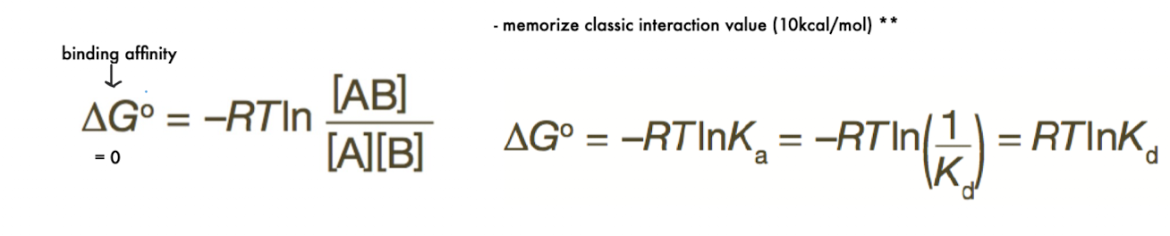
Dissociation Constant (K_D) & Binding Affinity

K_D​ is the ligand concentration at which half of the receptors are bound.

• Low K_D​ → high affinity (tight binding)

• High K_D→ low affinity (weak binding)

K_D​ is an inverse measure of binding strength.

Relationship between K_D and ΔG^∘

∆Gº = RT ln(K_D)

• more negative ∆Gº → stonger binding (low K_d)

• larger K_D → less favorable binding

• key idea: binding affinity is a thermodynamic property

• relationship b/w K_d and ∆Gº is logarithmic: a small energy change (e.g. one hydrogen bond) leads to a 10-fold change in K_d

Implications:

• Minor structural changes (e.g., side chains, H-bonds) can drastically alter binding

  • e.g. changes in amino acid side chains or in overall conformation can change the likelihood of two proteins binding to each other

• Enables fine-tuning of specificity in biological systems

Binding Specificity

Binding specificity is the ability of a protein to prefer one ligand over others.

• Determined by:

  • shape complementarity

  • chemical interactions (H-bonds, charges, hydrophobicity)

Variants can:

• reduce specificity → off-target binding

• increase specificity → more selective interaction

Binding Specificity Thermodynamics

• specificity depends on the difference in binding free energies between ligands

  • ∆Gº_B - ∆Gº_A

• If binding to B has more negative ΔG^∘ → B is preferred

• Larger difference → higher specificity

• Even small energy differences can strongly bias binding toward one ligand

Molecular force fields & minimization (MD basics)

• Force fields (FF): mathematical models describing atomic interactions

  • include bond, angle, electrostatic, and van der Waals terms

• Energy minimization:

  • adjusts structure to lowest energy conformation

  • removes steric clashes before simulation

Binding Equilibrium and K_d

• at equilibrium, the rate of binding equals the rate of dissociation: K_on[A][B] = K_off [AB]

• the dissociation constant is K_D = K_off / K_on = ([A][B])/[AB])

• stronger interactions shift equlibrium toward the complex (AB)

Fractional Occupancy

• Fractional occupancy describes the fraction of receptor (A) bound to ligand (B):

  • fractional occupancy = [AB]/[A]_total

• [A] = [AB] when half of A is bound to B

• using the equation from the previous slide, K_d = [B] under these conditions

• initially occupancy increases significantly, then levels off

Saturation and Binding Curves

• as ligand [B] conc. increases, occupancy rises rapidly at first, then levels off (saturates) as receptors become fully bound

• if [B] » K_d: system is saturated, nearly all receptors in bound state (AB)

• if [B] = K_d: 50% occupancy

• binding follows a saturation curve: fast increase → plateau when receptors are fully occupied

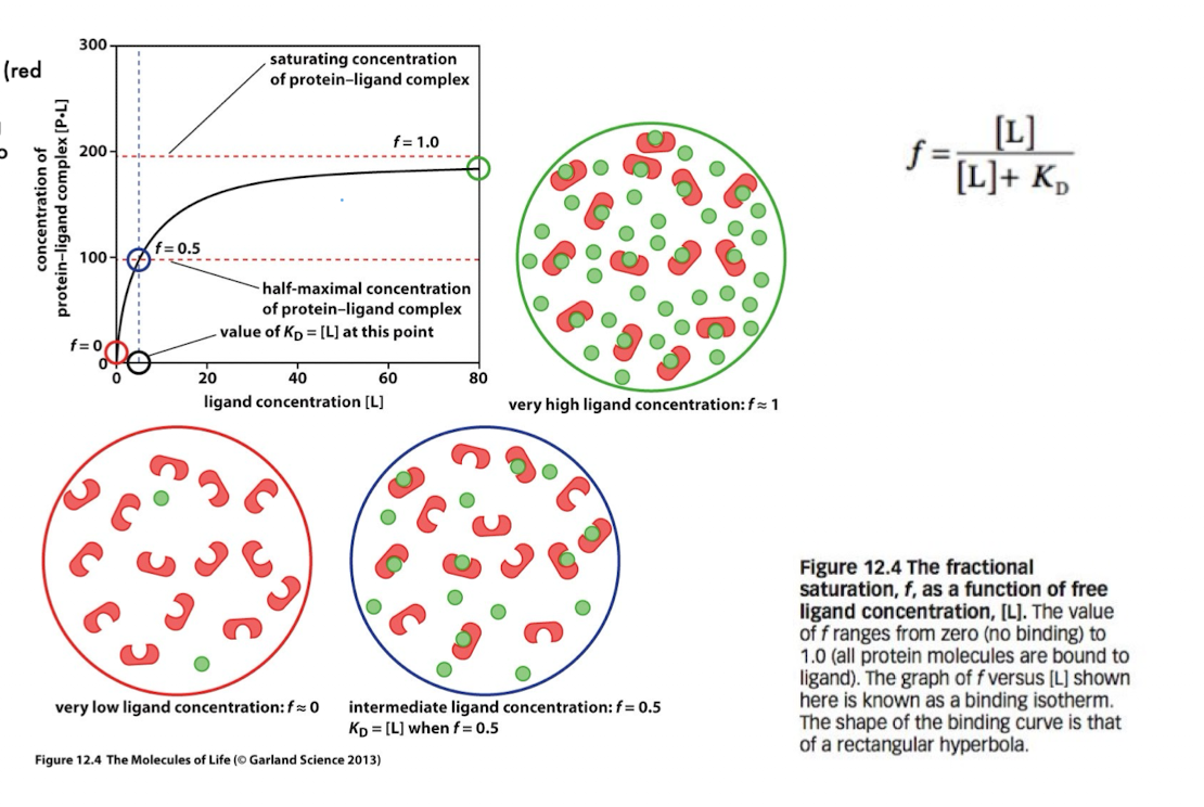
Binding Isotherm (fractional occupancy equation)

f = [L] / ([L] + K_d)

• f = fraction of protein bound to ligand

• [L] = ligand concentration

• f = 0 → no binding

• f = 1 → full saturation

• f = 0.5 when [L] = K_d

This equation describes how binding increases with ligand concentration.

Binding Isotherm Curve

The plot of f vs [L] is a rectangular hyperbola:

• Low [L]: very little binding (f≈0)

• Intermediate [L]: rapid increase in binding

• High [L]: saturation (f≈1)

Important point:

• At f=0.5 → [L]=K_D

Promiscuity

• off target interactions results from low specificity

How do ideal binding affinity and K_D​ depend on biological function? Case A

Permanent Complex

• the affinities of the partners are likely to be high

  • low K_d

  • binding is near saturation → stable complex

• importantly the dissociation constant is lower than the endogenous concentrations of the components so that binding will be close to saturation

  • K_d « cellular concentrations

How do ideal binding affinity and K_D​ depend on biological function? Case B

Signaling Complex

• affinities of partners are not so high

• dissociation constant is roughly equal/slightly higher than the endogenous ligand concentration

Why are weaker (moderate) affinities important for signaling interactions?

• allows small changes in either ligand conc. or other modulating factors to lead to big changes in the fraction of ligand bound

  • allows interaction to be regulated

• weaker affinities allow interaction to be more dynamic

  • K_d of an interaction is diefined by its off rate (K_off) divided by its on rate (K_on)

  • k_on is limited by rate of diffusion, k_off is limited by affinity

• higher k_off → shorter binding time, enables rapid signal termination and regulation

Why are weaker (moderate) affinities important for signaling interactions? Continued

In signaling systems (e.g., hormone–receptor like GLP-1R):

• If affinity is too high (very low K_D​):

  • receptors are nearly always saturated

  • small changes in ligand concentration produce little additional response

  • system loses dynamic range (no “sensitivity window”)

• If affinity is moderate ( K_D [ligand]):

  • receptor occupancy changes strongly with small ligand changes

  • system becomes highly responsive and regulatable

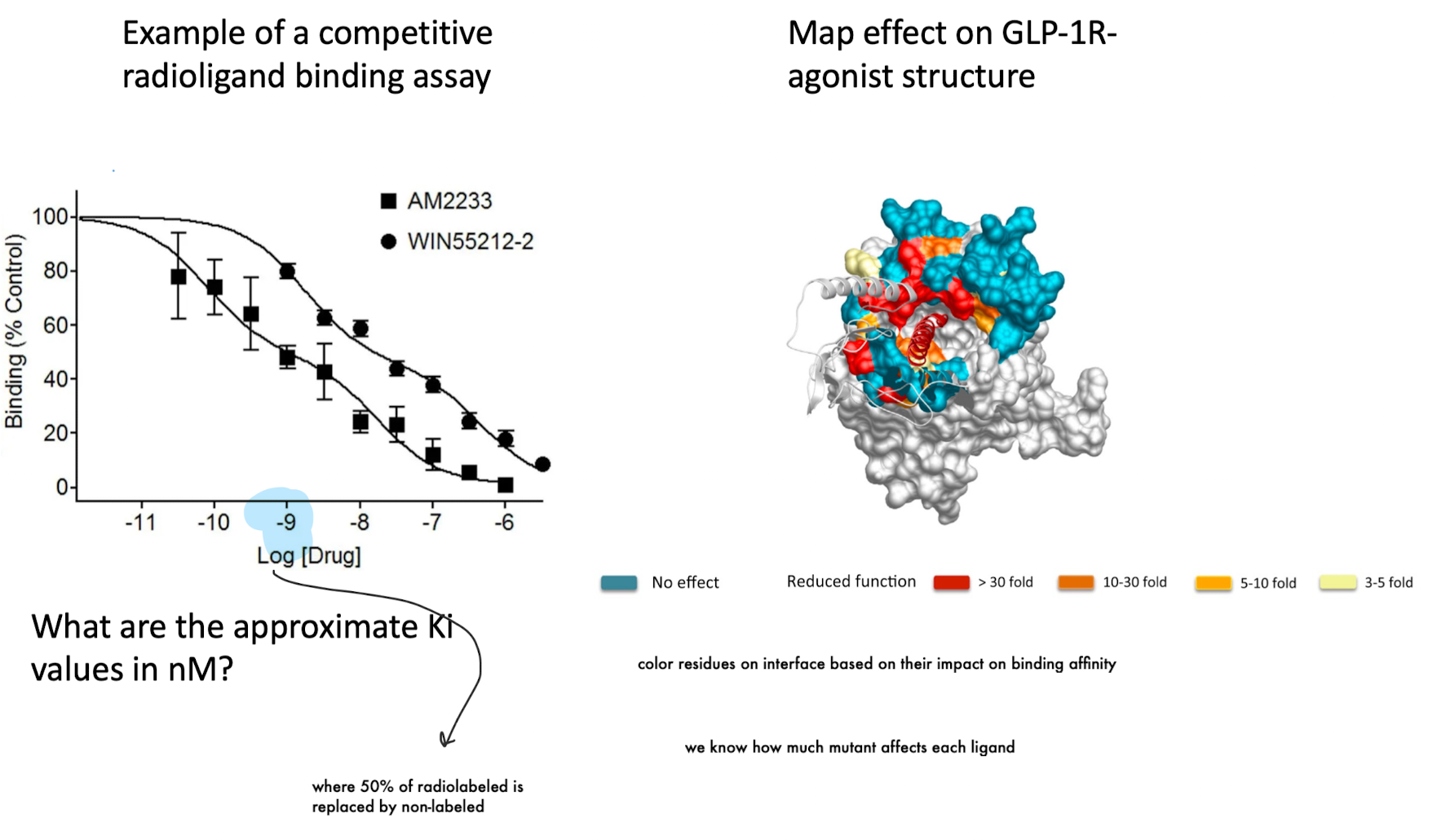
Competitive radioligand binding assay (how affinity is measured)

A fixed amount of radiolabeled ligand (e.g., ¹²⁵I-exendin(9–39)) is bound to the receptor, then increasing concentrations of an unlabeled test ligand are added.

• The test ligand competes with the radiolabeled ligand for receptor binding

• As test ligand concentration increases → radioligand binding decreases

• The concentration that reduces binding by 50% is the IC₅₀

Why are molecular dynamics simulations necessary instead of analytical solutions?

We cannot solve molecular behavior analytically because:

• biological molecules have too many atoms and interactions

• systems are too complex for closed-form equations

Instead,

• MD uses numerical (step-by-step) comparison

• calculates atomic motion over time, using physical force laws

What can we do w/ MD Simulations?

• protein structure and dynamics: MD simulations help study protein folding, conformational changes and stability

  • we can use them to calculate free energies

• enzyme mechanisms: MD cab help reveal atomic-level details of chemical reactions

• membrane dynamics: simulations can be used to investigate behavior of lipid bilayers and membrane-proteins interactions

• nucleic acids: they reveal the structure, flexibility, and interactions of DNA and RNA

• drug discovery: they are used to model protein-ligand interactions, optimize drug candidates

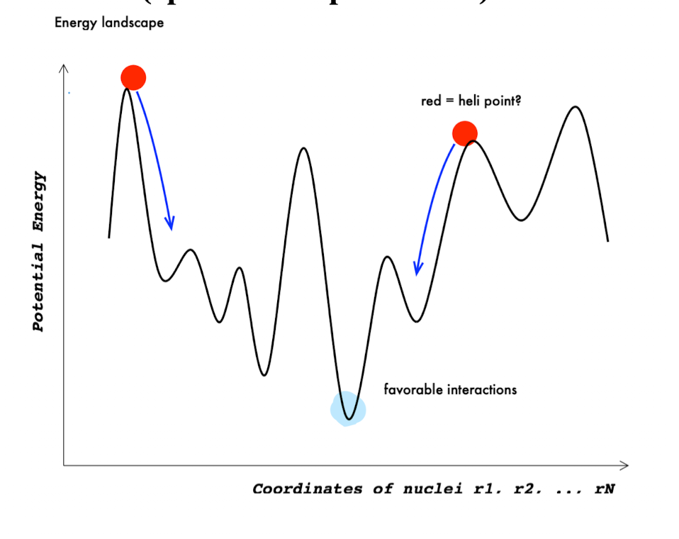
What do we need for MD simulations?

• an energy landscape (potential energy function) that describes how atoms interact

  • Defines forces between atoms (bonded + non-bonded interactions)

  • Includes effects of covalent bonds, electrostatics, van der Waals forces

  • Determines stable (low-energy) vs unstable (high-energy) configurations

• ways to move the landscape

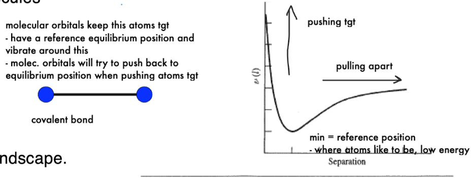
What does the molecular energy landscape represent physically?

• Atoms have a preferred equilibrium position (minimum energy state)

• Displacement from this position creates restoring forces

  • pulling atoms back together or pushing them apart

• Bonds and molecular orbitals act like springs maintaining structure

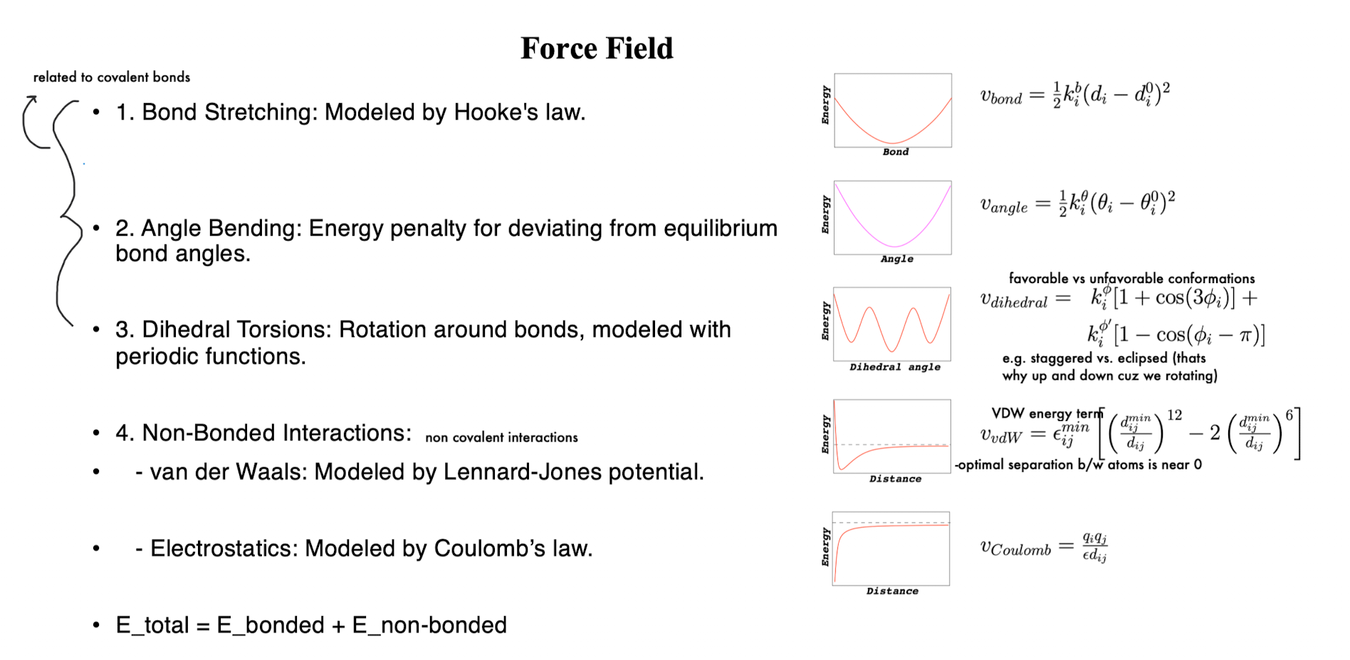
Force Field

• a set of mathematical functions and parameters used to model the interactions b/w atoms in a molecular system

• purpose: approximate the potential energy of a system based on atomic positions

• types of forces:

  • covalent: bonded (bonds, angles, dihedrals)

  • non-covalent (VDW, electrostatics)

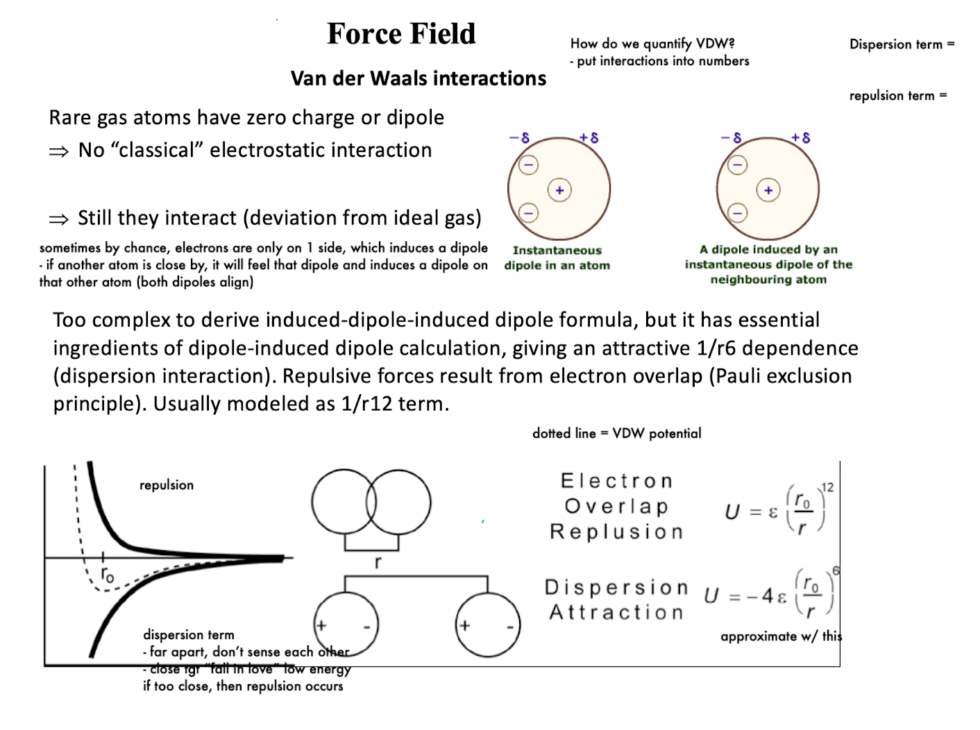
How are VDW interactions modeled in force fields?

• dispersion term: 1/r⁶; repulsion term (electron overlap/Pauli exclusion): 1/r¹²

• Far distance: no interaction

• Intermediate distance: attraction (“optimal binding distance”)

• Very close: strong repulsion (electron overlap)

• VDW interactions balance attraction (dispersion) and repulsion (Pauli exclusion) to define stable atomic spacing

Force Field: Reference Point

• the geometry where energy is lowest (most stable)

  • the further away, the higher energy penalty

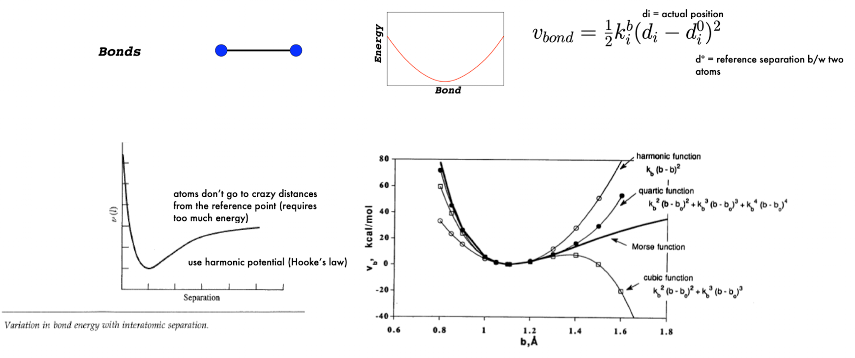
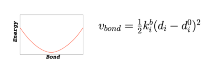
Force Field: Bond Stretching

• modeled like a spring: E = ½ k(r-r₀)²

• r₀ = ideal bond length (reference point)

• energy increases symmetrically if bond is stretched or compressed

• k = stiffness (steeper curve = harder to stretch)

• narrow/steep curve → strong bond

• wide curve → flexible bond

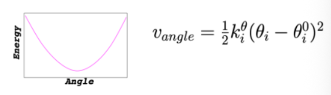
Force Field: Angle Bending

• minimum at equilibrium angle; energy increases as you bend away from ideal geometry

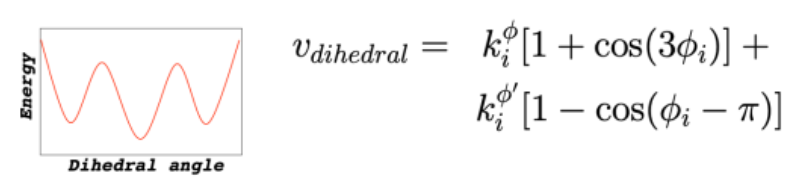
Force Field: Dihedral Torsions

• energy changes periodically as bond rotates

• multiple minima = multiple stable

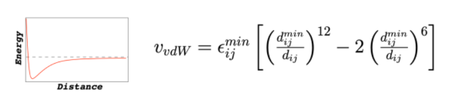
Force Field: Non-Bonded Interactions

• VDW (Lennard-Jones potential)

• V = potential energy

Interpret the curve:

• far apart: V ≈ 0 (no interaction)

• intermediate distance: negative energy (attraction)

• too close → sharp increase (repulsion), very high V

• sweet spot: minimum (most stable separation b/w atoms)

  • distance where attraction = minimum

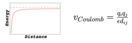
Force Field: Coulomb’s Law (Electrostatics)

• opposite charges → negative energy (attraction)

• same charges → positive energy (repulsion)

• Stronger charges / closer distance → stronger interaction

Force Field Parameterization

• process of deriving the parameters (bond lengths, angles, charges)

• methods: fitting to experimental data (e.g. crystals structures, spectroscopy)

• quantum mechanical calculation: how does energy change when pulling/pushing atoms tgt to get K

• Challengs:

  • balancing accuracy and computational efficiency

Limitations of Force Fields

1. Approximations in the mathematical model: interactions are simplified mathematical forms

2. Difficulty modeling:

• Polarizability.

• Complex chemical reactions.

3. Dependence on quality of parameterization: accuracy depends on how well force-field parameters are fitted to experimental data

4. Computational cost for large systems

What is energy minimization in molecular dynamics?

Energy minimization is the process of finding a stable (low-energy) molecular structure on the energy landscape.

• Atoms start in an initial configuration (often not optimal)

• The system is adjusted to reduce total potential energy

• Result = local energy minimum (stable conformation)

How is energy minimization in MD similar to linear regression?

Both are optimization problems:

• Linear regression: find weights www that minimize loss (error)

• MD energy minimization: find atomic positions that minimize potential energy

Analogy:

• weights www ↔ atomic coordinates

• loss function ↔ energy function

• best fit line ↔ lowest-energy structure

Why can’t energy minimization in molecular systems be solved using standard calculus?

In molecular systems:

• Energy depends on many variables (x, y, z for every atom)

• There are many interacting terms simultaneously (bonds, electrostatics, VDW, etc.)

• Improving one interaction can worsen another

Because of this:

• you cannot simply take derivatives and solve analytically like in simple functions

• the system is high-dimensional and highly coupled

How is energy minimization performed in molecular dynamics simulations?

Energy minimization is done using numerical optimization methods:

• Start from an initial structure

• Move atoms in small iterative steps

• Always move “downhill” in energy

Limitations:

• only finds a local minimum (closest low-energy state)

• does NOT guarantee the global minimum (lowest possible energy)

• different starting points can lead to different results

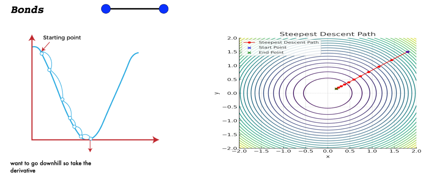
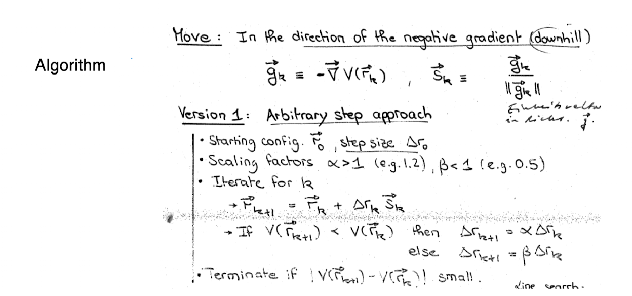
Gradient (Steepest) Descent

• the steepest descent method minimizes a function by moving iteratively in the direction of the steepest negative gradient

• key idea is to minimize a function by following the direction of maximum decrease

• At each step, compute the gradient (slope) of the function

• Move in the negative gradient direction (downhill)

• Repeat until reaching a minimum

Steepest Descent Method: Advantages vs Limitation

Advantages: simple and intuitive, effective for small-scare minimizations

Limitations: convergence can be slow near minima

How steepest descent works?

• compute gradient ∇(x_k) at the current point r_k

• choose direction: move in the direction -∇(x_k)

• choose step size: ⍺_k determines how far to move

• update position: X_k+1 = x_k - ⍺∇f(x_k)

How does steepest descent relate to energy minimization in molecular systems?

• Start with a molecular structure

• Use a force field to compute energy

• Compute the gradient of energy → gives direction of force

• Move atoms in direction that lowers energy