Labour Economics
1/77
There's no tags or description
Looks like no tags are added yet.
Name | Mastery | Learn | Test | Matching | Spaced | Call with Kai |
|---|
No analytics yet
Send a link to your students to track their progress
78 Terms
Labour Economics
A branch of economics that studies how the labour market works by focusing on participants and their dynamics
What are the stocks in the labour market?
> Children - Aged 0-15
> Employed - 16 or over and work a min 1 hour a week
> Unemployed - 16 or over who don't work but are seeking work
> Economically inactive - 16 or over who don't and aren't actively looking for a job
Why have the type of male jobs changed?
> Technological change - manufacturing becomes capital-intensive
> Demographic - e.g. higher education = more skilled or service-based roles
> Globalisation - most primary and secondary sector jobs have been offshored to developing countries
Developments in the UK labour market
> Structural change - Mining and manufacturing jobs down 90% by 2020 (impacted male employment)
> Changes in types of jobs for men - fewer employed in manual jobs
> Changes in types of jobs for women - mostly employed in high-skilled/low-skilled social jobs
> Changes in wages - Since 1980 - 90th percentile wages increased more rapidly, creating wage inequality with the 50th and 10th percentile
Firm decisions during labour market recessions
> Lay off workers
> Delay or cancel hiring
> Reduce hours of work
> Reduce pay
Workers decisions in labour market recession
> Don't leave current job
> Stop searching for new jobs - become "inactive" or "discouraged"
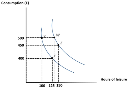
Consumption and Leisure Indifference curves
They represent the trade-offs between consumption and leisure to preserve the same level of utility
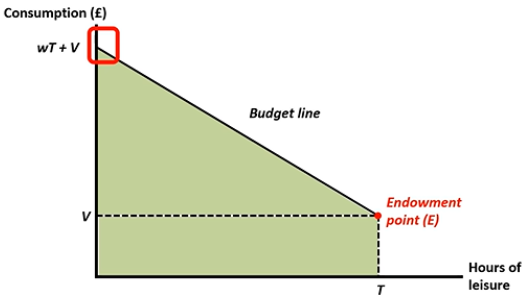
The budget constraint
C = wh + V
working hours x wage
other sources of income
L = T - h - For an hour of work, an individual sacrifices an hour of leisure
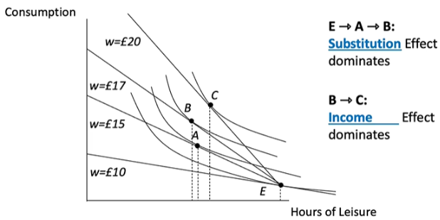
Income Vs Substitution effect
Income effect - overall income increases, allowing them to buy more things → Leisure becomes more attractive
Substitution effect - wage rate increases, making an hour of leisure relatively more expensive (increases opportunity cost).
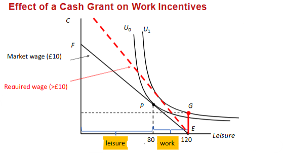
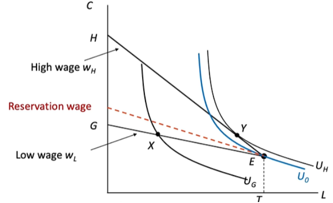
Effects of a Cash Grant
1) The individual is originally on point P but then has to stop working (e.g. disability) and therefore goes to point E
2) The government then offers a cash grant that puts him on point G and also a higher indifference curve (U1)
3) To get back into work, the individual needs to be offered a new wage that brings him tangent to the new indifference curve
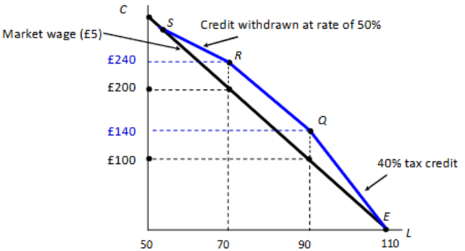
Effects of the earned-Income tax credit on the budget constraint
Eligible groups: Single Mothers
Basic components:
Zero income: no credit paid
Low income: top-up for every dollar earned - negative income tax
A bit higher income: constant total credit
Still higher income: total credit decreases
High income: no credit paid
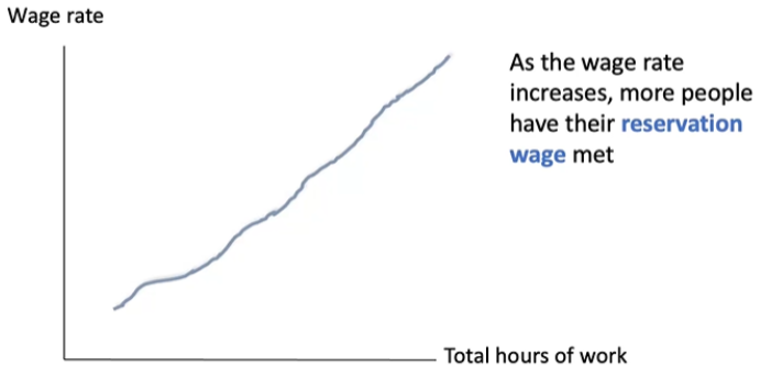
Reservation Wage
The reservation wage is the lowest wage rate that leaves an individual indifferent between working and not working.
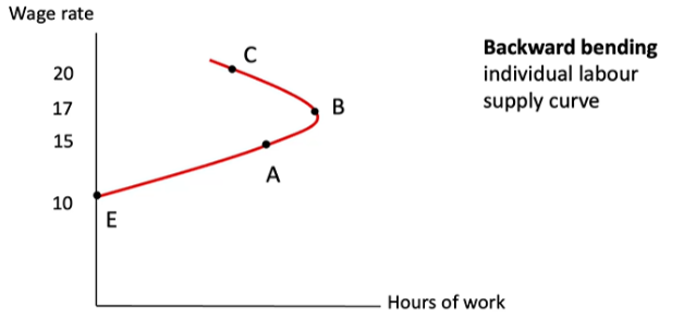
The Individual Labour Supply Curve
Backward bending individual labour supply curve
Derives from the points shown in the Individual labour supply curve. Shows how as the wage increases, the income effects begin to dominate.
The aggregate labour supply curve
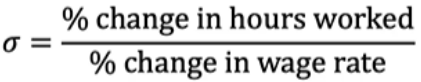
The elasticity of labour supply
> Measures the extent to which hours worked change in response to a change in the wage rate
> less than 1 = labour supply inelastic, greater than 1 = labour supply elastic
> Less than zero, labour supply curve is downward sloping (income effect dominates)
> More than zero, labour supply curve is upward sloping (substitution effect dominates)
Randomised Social Experiment
> Select a representative sample
> Randomly assign study subjects to a “treatment” or a “control” group
> The advantage is that treatment and control will be identical (on average) along all other dimensions. The treatment is thus exogenous, which allows us to “identify” a true causal effect.
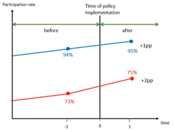
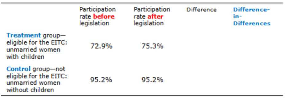
Before and After Comparison (Difference-in-Differences)
> Key assumption: The growth trend in participation rates between the two groups of women (with vs without children) would’ve been the same
> After the policy, the participation rate of women with single children increased at a faster rate
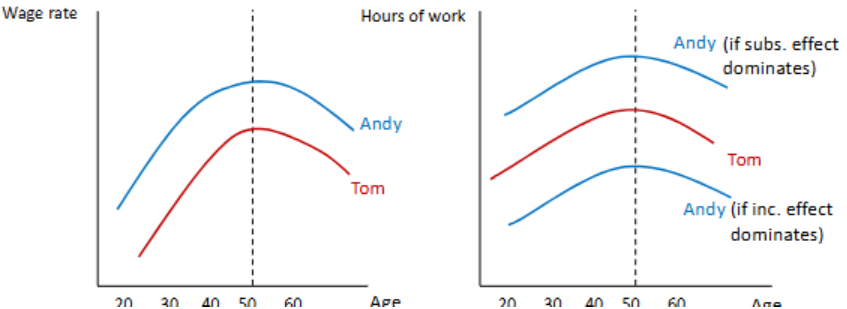
Hours of Work over the Life-Cycle for Two Workers with Different Wage Paths
Andy earns more than Tom.
> If the substitution effect dominates, Andy will work more hours at a higher wage
> If the income effect dominates, Andy will work fewer hours at a higher wage
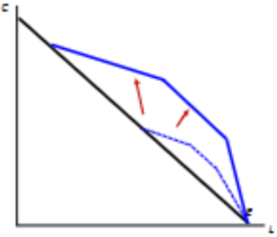
Evaluation of the EITC (Earned Income Tax Credit) expansion
> Treatment group: single women with children (no income from spouse)
> Control group: single women without children (not eligible for EITC)
> Impact on labour supply for single women with children shown in the graph:
Raises income for low earners → shifts budget line up.
Phase-in encourages more work; plateau provides constant support; phase-out reduces credit gradually.
Overall → increases labour supply.
Elssa and Liebman study (1996)
> They studied the effect of an expansion of the EITC on labour supply
> Labour force participation of single mothers increased after the expansion of the EITC by an additional 2.4 percentage points
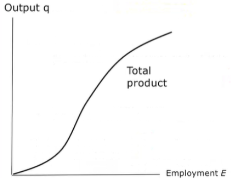
Total product of labour curve
> Output increases as employment increases (at a diminishing rate)
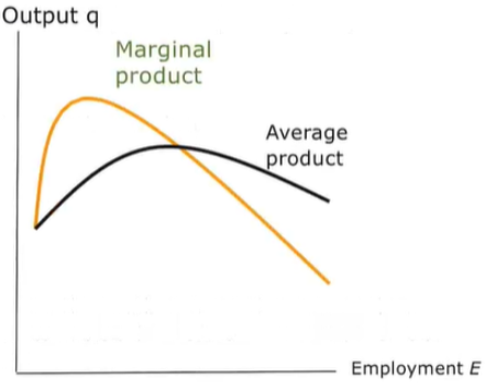
Marginal and Average product curves
> MP curve: Shows the additional output from hiring one more unit of labour. Initially rises due to specialisation, then falls due to diminishing returns.
> AP curve: Shows output per unit of labour . Rises at first, reaches a maximum, then declines as diminishing returns set in.
> MP intersects AP at AP’s maximum point.
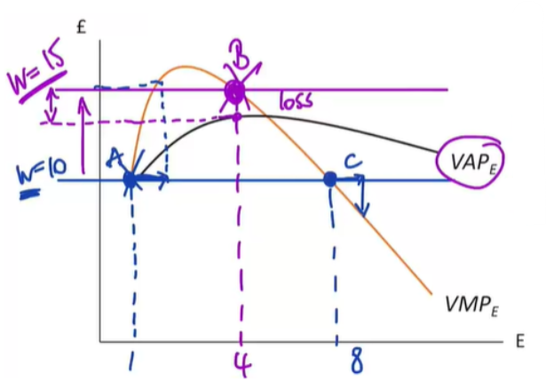
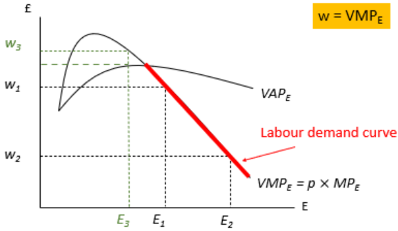
The Employment decision in the short run
The firm employs labour up to the point where VMPe = w
Profit maximisation also requires that the VMPe is declining so we are at point C and not point A
The wage will always be less than or equal to VAP
Short-Run Labour Demand Curve
Employment decision in the Long Run
> In the long run, all inputs can be changed
> An isoquant is used that describes all combinations of K and E which produce the same level of output
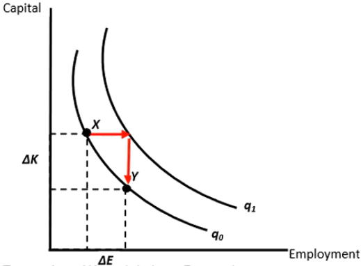
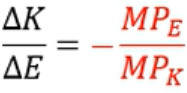
Slope of the Isoquant
> How much capital is needed to replace each unit of labour without a decrease in production
> The ratio is called the marginal rate of technical substitution (diminishing between E and K)
In what two ways do firms decided how many workers to hire in the long run?
> Cost minimisation - find the least costly combination of capital and labour to produce a chosen level of output
> Profit maximisation - find the most efficient combination of capital and labour at a chosen level of costs
What is the impact of a wage decrease on the long-run demand for labour?
> Scale Effect - Firm takes advantage of cheaper labour by expanding production
> Substitution effect - Firm takes advantage of the wage change by rearranging its mix of inputs (i.e. output stays constant, employment increases, and capital decreases)
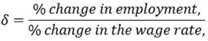
Elasticity of Labour Demand
> Measures the extent to which employment changes in response to a change in the wage
> If 0 > δ > -1, the elasticity of labour demand is inelastic
> If δ < -1, the elasticity of labour demand is elastic
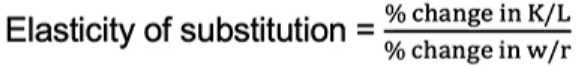
Elasticity of substitution
> Measures how easy it is to replace one input (labour) with another (capital)
> K/L - capital-labour ratio
What are Marshall’s 4 rules of derived demand?
Labour demand is more elastic the greater the elasticity of substitution
Labour demand is more elastic the greater the elasticity of demand for the output
Labour demand is more elastic the greater labour’s share in total costs
Labour demand is more elastic the greater the supply elasticity of other factors of production
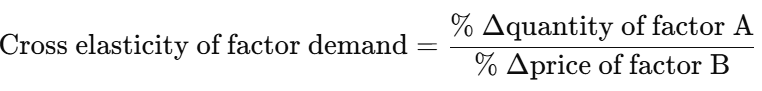
The Cross-Elasticity of Factor Demand
Measures how the demand for one input changes when the price of another input changes
How do you determine if two inputs are substitutes or complements?
> Two inputs are substitutes if:
The cross-elasticity is positive
The elasticity of substitution between the two inputs is large
> Two inputs are complements if:
The cross-elasticity is negative
The elasticity of substitution between them will be small
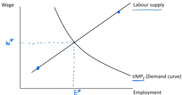
Perfectly competitive labour market
> Profit maximisation point in a perfectly competitive labour market is where labour supply = VMPe
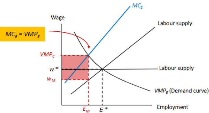
Labour market Monopsony
A single employer faces an upward-sloping labour supply curve, meaning the supply of labour to the firm is relatively inelastic, giving the firm wage-setting power and allowing it to pay wages below the competitive level (employees won’t leave for a small wage increase).
Imperfectly competitive labour market (Monopsony)
> A firm operating in a monopsony would employ fewer workers and also pay a lower wage, but the value each worker brings in is higher
> The profit maximisation point is when MCe = VMPe and the profit is VMPe - Wm
Labour supply frictions
> These are frictions that cause labour markets to not be perfect:
Cost of searching for new job opportunities
Cost of training
Cost of moving to a new area
Risk when quitting a job
Labour demand frictions
Fixed cost of hiring:
Selection Costs
Training
Fixed cost of firing
Cost of moving to regions with lower labour costs
Overtime versus a new worker
Increase in labour productivity
1) VMPe curve shifts out
2) This increases both the wage and employment (in competitive only employment)
Comparison between perfect competition and Monopsony
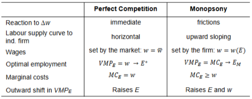
Empirical Evidence - Supply of Nurses to a Hospital
> Before 1991 - Nurses in VA hospitals were paid according to the national scale instead of location in terms of cost of living
> Nurse Pay Act (1990) - tied VA wages to the wages of the local labour market conditions
> This increases wages and increases employment (elasticity of labour supply = 1), in line with the idea of a monopsony labour market.
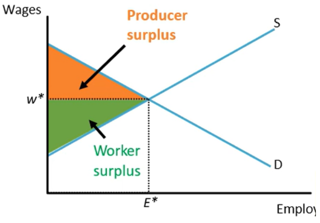
Labour Market equilibrium
Producer surplus - if E* is 10, then the first 9 workers have a value of marginal product higher than w*.
Worker surplus - w* being higher than the reservation wage
Wage pressures will always bring the wage back to equilibrium.
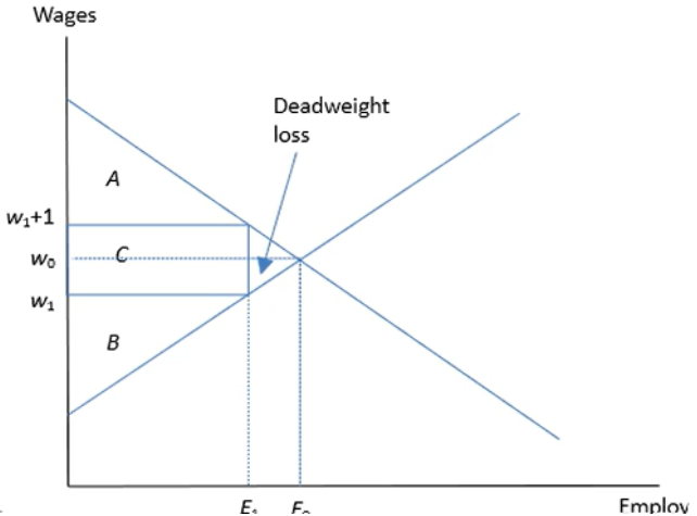
Payroll Taxes
These create a “wedge” between the price paid by firms for workers and the income the workers actually keep, in turn affecting the supply and demand for labour.
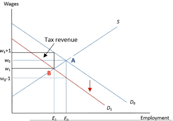
Payroll tax on firms
> Increases the cost of hiring a unit of labour for the firm, shifting the Demand curve down
> The new equilibrium wage is w1 + the new equilibrium employment is E1 (Point A to B)
> The firm, however, is paying the wage w1+1
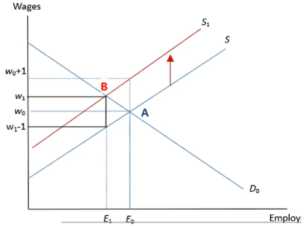
Payroll Tax on workers
> Increases the cost of working for workers, shifting the Supply curve up
> The new equilibrium wage is w1 + the new equilibrium employment is E1 (Point A to B)
> The workers, however, receive an actual wage of w1-1
Deadweight loss of Payroll Taxes
> A = Producer Surplus
> B = Consumer Surplus
> C = Government Revenue
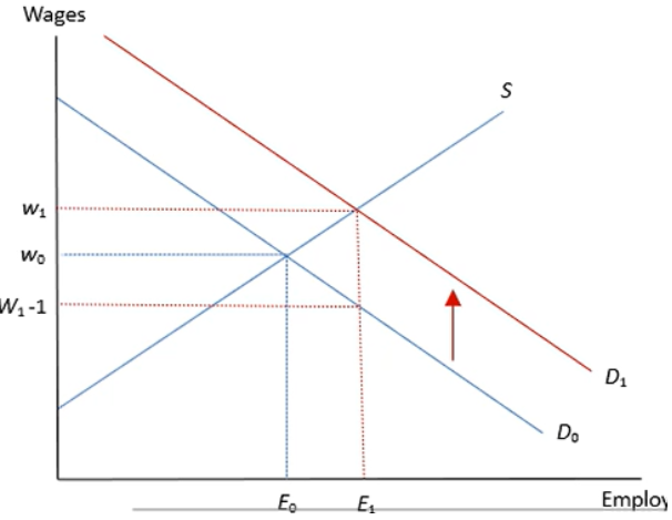
Wage Subsidies
> Shifts the Demand curve up
> Both wages and employment increase to w1 and E1
Minimum Wage on the Market Equilibrium
According to this model, the minimum wage would cause unemployment; however, this is unrealistic, and it doesn’t really occur in real life.
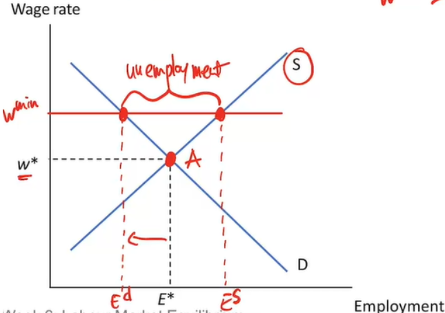
Minimum wage in a perfectly competitive market
How many workers lose their jobs is determined by the elasticity of labour demand
If > 1, then the job losses will outweigh the gain in wages and welfare will be lower
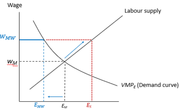
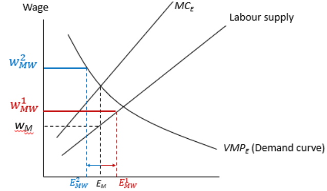
Minimum Wage on a Monopsonistic Firm
> Monopsonist firms hire at point B (MCe = VMPe) and pay wages at Wm
> A minimum wage (Wmw1) is implemented above the wage paid by the firm, which increases employment to Emw1
> However, if the minimum wage were implemented at a too high rate (Wmw2) then employment would decrease to Emw2
Card and Krueger (1994) - employment in the fast food industry
> Treatment group - New Jersey (they increased the state minimum wage from $4.25 to $5.05)
> Control group - Pennsylvania (did not change their minimum wage)

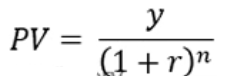
Present Value in N years
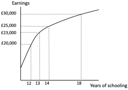
The Wage Schooling Locus
Describes how much is earned at different levels of schooling
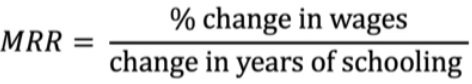
The Marginal Rate of Return to Schooling
Measures the percentage change in earnings resulting from an additional year of schooling
Each additional year of education leads to a smaller salary increase
Each additional year of education increases the cost of staying in school
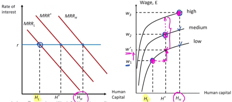
Workers differ in the MRR of education
MRR = R - individuals invest in education if its returns are equal to any other investment
The market pays individuals with more ability higher wages regardless of their years in education
Even with longer education, low-ability workers would still earn less than higher-ability workers.
Higher-ability workers benefit doubly: they earn higher wages and tend to stay in school longer, which further increases their earnings.
Solution to the Ability Bias
> Studies of twins
Identical twins have similar innate ability (should be on the same wage locus)
Compute the % wage difference per year of schooling between twins
A study for the UK uses data from St Thomas ' Hospital “Twin Registry”.
It compares the wages of 428 identical twins (Bonjour et al. 2003)
Finds that the return to education is not strongly biased upwards, which strongly supports the theory of human capital
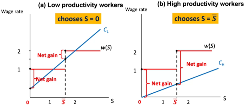
Schooling as a signal
Schooling does not increase a worker's productivity but sends a “signal” about that person’s innate ability (productivity)
More expensive for low productivity workers to acquire the signal
Low productivity workers vs high productivity workers gains from university
The net gains from attending university for low-productivity workers are not as significant as the net advantages high-productivity workers gain from higher education.
General vs Specific human capital
> General human capital increases productivity in any job or firm
> Specific human capital increases productivity only in a particular job or firm
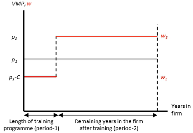
2-period model of general human capital training
Beckers (1962) - firms have no incentive to pay for the cost of general training. If they did, other firms could “poach” the trained worker.
Workers, therefore, pay by accepting a lower wage (w1) during the training period
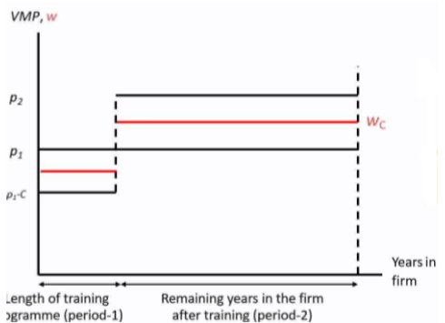
2-period model of specific human capital training
Becker (1962) - specific training occurs only if costs and returns to investments are shared between the firm and the worker
With specific training, neither firms nor workers have an incentive to break the employment contract in the post-training period:
Firms are paying workers less than the value of their marginal product
Workers are earning more than they would at another firm
Stevens (1994)
Training is never purely general: instead, “transferable” training (which raises productivity in a limited set of firms) is far more realistic. This shows why firms do pay for general training (e.g. MBA programmes).
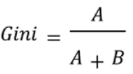
The Gini Coefficient
Measures how much the distribution of income among individuals deviates from a perfectly equal distribution.
If the richest household had 100% of the income, then the Lorenz “curve” would be a right-angle and B = 0, so the Gini coefficient would be 1
Therefore, a higher Gini coefficient implies more inequality
What are the 2 reasons argued by Neoclassical labour economics for wage differences?
1) Productivity differences - e.g. younger people tend to earn less due to less knowledge and experience
2) Differences in the rewards paid for different skills
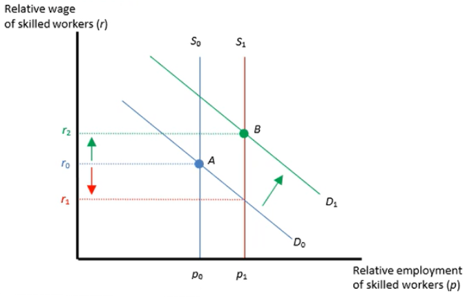
Supply and Demand for skilled workers
1980s - increase in the supply of skilled workers (S0 to S1) should’ve decreased the wages of skilled workers.
However, due to the even greater shift in demand for skilled workers, wages rose.
What are the 4 suspect for the increase in earnings inequality?
1) Globalisation
2) Technological change
3) Labour market institutions
4) Supply of different groups of workers
Globalisation
Heckscher-Ohlin model - Developed countries export skill-intensive goods and import unskilled labour-intensive goods.
Trade thus increases the demand for skilled workers in developed countries.
Higher demand for skilled workers raises their wages relative to unskilled workers, widening the wage gap and increasing wage inequality.
Technological Change
Technology is skill-biased: it’s a substitute for unskilled labour, and a complement for skilled labour
If skilled workers use computers more, introducing computers will raise the skilled-unskilled wage ratio.
Dinardo & Pischke (1997) - Even basic "white-collar" tools like pencils and chairs have a wage premium.
Institutional Change
The US and UK experienced much larger increases in wage inequality because of:
Declining trade unions → workers have less power to negotiate pay → low and middle wages fall behind
Weaker/eroded minimum wage → the lowest-paid workers earn relatively less
Reduced public sector employment → fewer stable jobs with similar pay levels → private sector jobs have bigger pay differences
Job Search Model assumptions
1) Workers are identical
2) Workers know the wage distribution, but not which firms are offering which wage
3) Workers prefer a higher wage to a lower wage
4) The costs of search are significant
What are the two strategies/models for the maximisation of wages?
1) Non-sequential search model - the optimal sample size rules (Stigler, 1962) - solves the problem of what is the optimal number of job applications to make?
2) Sequential search model - the optimal stopping rule (McCall 1971) - solves the problem: what is the optimal wage offer which makes the job-seeker indifferent between acceptance and continued search?
The Optimal Stopping Rule for Wage Offers
> The worker must decide either to accept or reject incoming job offers
> Decision rule - accept only if wage is at least as high as the reservation wage (wr)
> Trade-off - waiting increases the likelihood of getting a better offer, but waiting is costly (time is money)
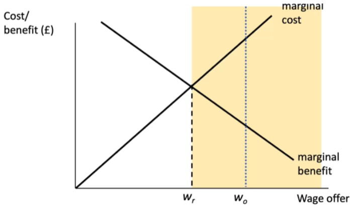
Marginal Costs and benefits of search
> Marginal cost of search - opportunity cost of foregone wages → increases with wages (+ Direct search cost)
> Marginal benefit of search - the probability of getting a better-paid job → decreases with wages
The Optimal stopping Rule
What factors does the marginal benefit of search depend on?
Assuming no more search once the job is found:
1) The number of job offers in the next period (+ with marginal benefits)
2) The probability of receiving a better-paying job offer (+ with marginal benefits)
3) The expected additional wage of a better-paying job offer (+ with marginal benefits)
4) The discount factor (how impatient you are) (- with marginal benefits)
What factors are the reservation wage determined by?
1) The benefit level, b (+ relationship)
2) The job offer arrival rate (+ relationship)
3) The discount rate (- relationship)
4) The position and shape of the wage distribution (- relationship)
What does the average unemployment duration depend on?
1) The reservation wage - the higher the wr, the longer the unemployment duration
2) Availability of jobs - more jobs available, unemployment duration falls (however, individuals respond by increasing wr so final result ambiguous)