Quantitative analysis

What information can be obtained about receptors?

• The affinity of drug-receptor interactions  

• The number of binding sites —> need to be able to spot additional binding sites to interpret data correctly 

• Pharmacological properties 

• Structure function relationships derived from pharmacological profiles 

• However, things like radioligand studies cannot give us information about receptor efficacy 

How?

• Incubate the tissues, cells etc with radiolabelled ligand 

• Separate the free drug from the bound drug by centrifuge or filtration (most of the time) because there will be no difference in the signal of a radioligand whether bound or free. With fluorescence we may be able to just look at the signal from the bound ligand without separating the free ligand 

• Estimate the amount bound at different concentrations of ligand 

  • Keep the amount of receptor constant but vary the amount of ligand to try and vary this profile 

• Use other drugs to displace the ligand to characterise the pharmacology  

• Introduce mutations into receptor protein to investigate structure function

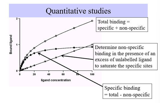
Interpreting results

• Total ligand binding curve will not saturate because this contains specific and non-specific ligand binding (ligand sticking to plastic ware or embedded in memb) 

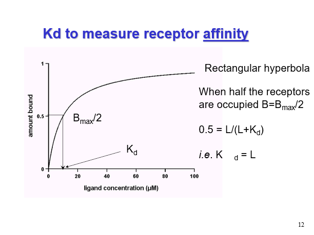
• Specific binding will saturate and will be a rectangular hyperbole shape which will also give us info about the affinity (Kd) and receptor density (Bmax)  

• Lowest Kd will be the tightest binding 

 

Why bother with quantitative analysis

1. Pharmacological profiling (can separate ligand binding for receptor subtypes) 

2. Identification and isolation of receptors 

3. Quantifying receptor number 

Analysis of binding data

Assume:

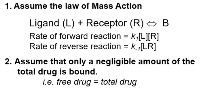
• Once we’ve reached equilibrium, the rate of the forward reaction is equal to the rate of the reverse reaction k1[L][R] = k-1[B] 

• Because we use such an excess of ligand on a very small concentration of receptors we are able to make the second assumption  

Equilibrium constants

• We use disassociation constant rather than association constant (Ka)  

• Equilibrium association rate = k1/k-1 = Ka, dissociation rate constant = k-1/k1 

• The reason that we chose kD because kA has units of litres per mole while kd has units of mol/L (molar) which is easier to understand and relate bac to our ligand binding experiments 

At equilibrium  

 

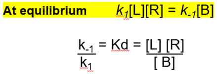
Equilibrium constants to measure affinity

• On the right is is we think of Kd at equilibrium whereas on the right is in terms of rate constant 

• The issue is that we don’t often know the concentration of receptor to calculate the kD  

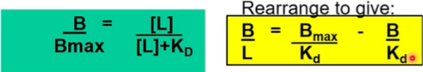
• So in order to take out the term [R] we can substitute this for Bmax – [B] 

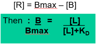
• This equation applies for simple bimolecular interactions between a ligand and its receptor 

Plotting ligand concentrations against bound ligand

Bmax

• Gives us the total number of receptors that you’ve bound in that experiment (total receptors) 

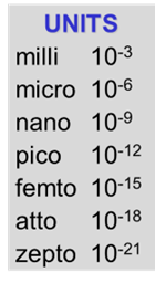
• Typically 10^-12 to 10^-15 moles/mg of protein which gives you a window to check for in your calculations 

Specific activity

• Is the amount of radioactivity of a particular radionucleide per mole of radioligand 

• So if we know the specific activity of a radioligand we can use this to sovert back to a concentration of ligand that must be bound 

Example of data

Example is of H3 spiroperidol binding to pig striatal membranes 

 

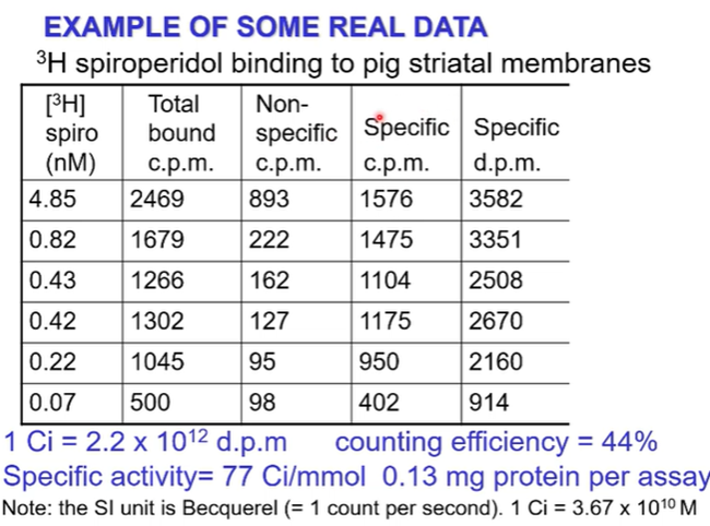
• Column on the left is the radioligand in nM across a range of concentrations as you go down. You then separate out the bound from the free and measure the bound with a scintillation counter, recorded in the second column (counts per minute)  

• The experiment will then be repeated, flushing with non specific cold ligand to ascertain how much non-specific binding there is (recorded in the third column)  

• Now subtract the non specific from the total bound to have specific bound (fourth column) —> this is the data that we’re interested in but its still in cpm  

• The machine that we count radiation is not 100% efficient at recording all the radiation. We need to take the counting efficiency into account —> in this case is 44% so if there were 100 radioactive particles would only count 44 of them 

• To convert between dpm (disintegrations per minute) to cpm we multiply by the counting efficiency  

• Dpm is the actual amount of radiation being emitted per minute 

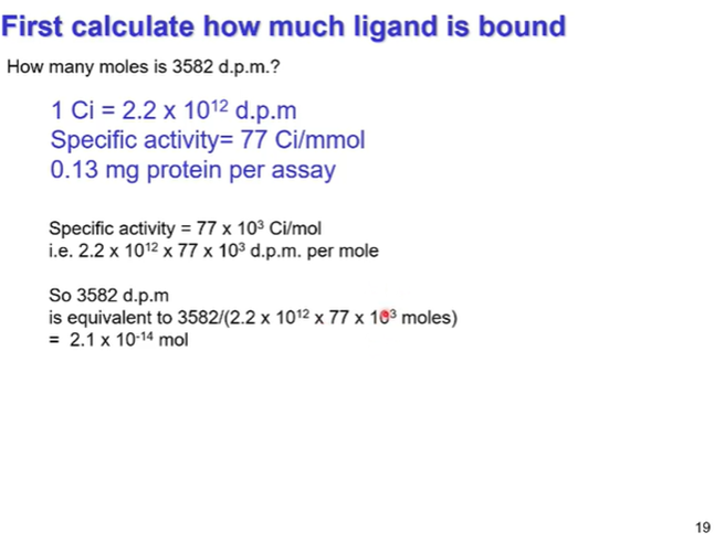
• With every ligand that is bound we get information about the specific activity in curies per mmol but our data is in dpm (disintegrations per minute)  

• To covert between these 1 Ci (curies) = 2.2 x10^12 dpm  

How to find Kd and Bmax

• Will always be told the conversion between curies and dpm, the specific activity in ci/mmol and the amount of protein er assay.  

Summary of working out ligand binding

• Add varying concentrations of radioligand  

• Record total bound in scintillation counter which gives counts in cpm  

• Then flood with cold ligand to assess non-specific binding and subtract that from the total to give you specific binding  

• Then account for the counting efficiency of the machine (cpm→dpm)  

  • E.g: if this is 44% then divide by 44 and x100 to go from cpm to dpm  

• Convert our dpm value to curies (1Ci Is 2.2x12^12 dpm)  

• We are given the specific activity of the ligand in curies per mole (Ci/mmol) so will have to work out how much protein is bound based off the number of curies emitted by the radioligand 

  • Specific activity is in Curies/mmol so convert to to curies/mol by x1000 

  • Dpm/ (2.2x10^12 x specific activity in mol) = moles of ligand bound 

• Moles of ligand bound/milligrams of protein to give us femtomoles per milligram of protein  

Plotting data

Direct plot

• Bound ligand in femtomoles per milligram on the y axis, concentration of radioligand on the x axis 9 (nM)  

• We observe a rectangular hyperbole → this is known as a direct plot  

• Some of the benefits of the direct plot is that it doesn’t require any modelling, data transformation and there’s no distortion of data points 

• But one of the limitations is that to accurately calculate Bmax you need the receptor to be fully saturated which requires very high ligand concentrations (around 100x the Kd) 

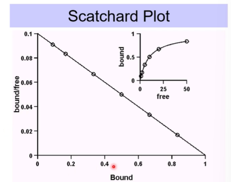
Scatchard plot 

• Easily linearise the data using the scatchard equation  

• Another method is the Lineweaver Burke plot but this is less favoured compared to the Scatchard plot 

• A plot of bound/free against bound should give us a straight line which has a slope of -1/kd and the x intercept should give us Bmax 

 

• Will usually give us a line of best fit, not always perfect data  

• Can extrapolate this slope to reach the x axis  

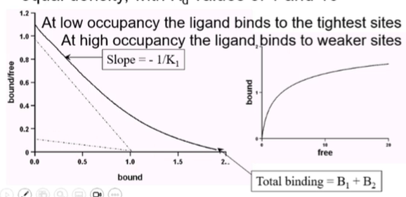
What if we don’t get a straight line?

• If our scatchard plot is slightly curved might indicate 

  •  more than one binding site (site heterogeneity)  

  • Negatve cooperativity 

• The curve should have two distinct phases:  

  • At low concentration a slightly linear portion  

  • At high concentration of free ligand a second linear portion with a different gradient  

• At low occupancy, the ligand will bind to the low-affinity site but at higher concentration there’s a second site with a weaker affinity which is occupied  

• We would not be able to interpret this from a direct plot 

• To calculate Bmax we draw a tangent and extract a Bmax for both portions and then add them together 

How deformed does it have to be?

Depends on the difference in affinities of the two binding sites → binding sites with small differences in affinity will be less deformed 

Negative cooperativity

• Can also be indicated from a bent looking Scatchard plot because binding of the ligand induces a conformational change which alters the affinity  

• Typically an agonist  

• Rarely see positive cooperativity in receptors 

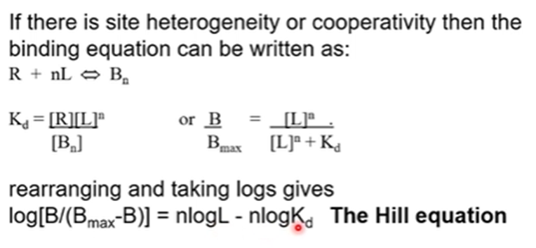
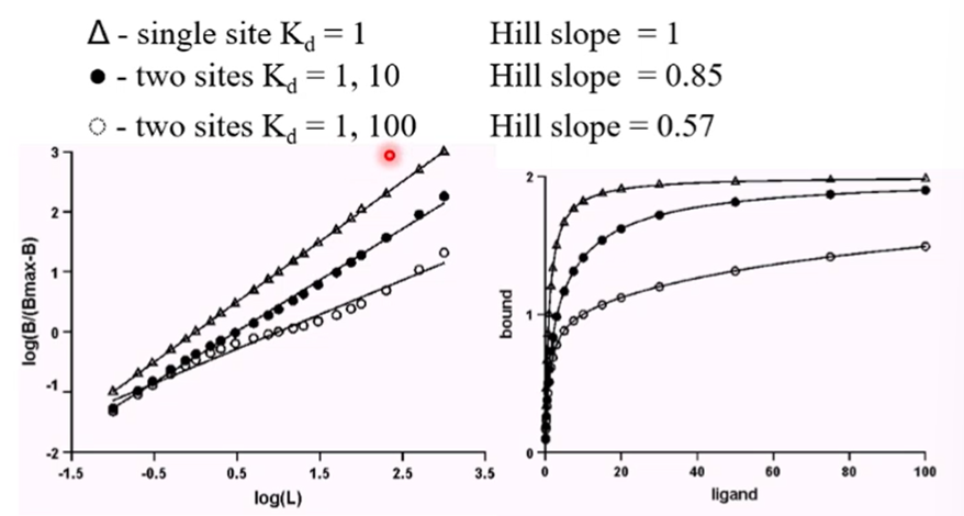
Hill plot

• If we suspect that there may be site heterogeneity or cooperativity then we can do the Hill analysis 

• Can tell us about the number of binding sites and whether they display cooperativity  

• To plot this then we would plot log[B/Bmax-B] against logL which will give us a straight line with the slope of n which is the Hill coefficient 

• If we have a single site with a kd of 1 then we will have a hill slope of 1  

• If we have a hill slope less than 1 it is indicative of site heterogeneity  

• The smaller the hill slope is the greater the difference is between the Kd of the binding sites 

Displacement curves

• Can use displacement curves to charcaterise a panel of other ligands 

• Have a fixed concentration of radioligands in the assay and can displace this with different amounts of an unlabelled ligand 

• Plot log of unlabelled ligand on the x and amount of ligand bound on the y 

• May not always reach zero 

• Want to know the conc of ligand that displaced half of the bound ligand which gives us an Ic50 of the second unknown ligand 

• Useful if we are unable to radiolabel the radioligand under investigation  

• IC50 is dependent on the concentration fo the labelled ligand and its Kd  

• Can then use the Cheung prusoff equation which corrects for this and calculates the equilibrium dissociation constant for the inhibitor Ki 

 

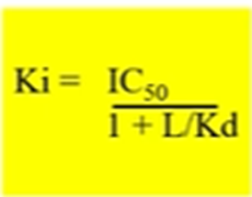
• Bottom half of the equation relates to the radioligand concentration and the radioligand Kd 

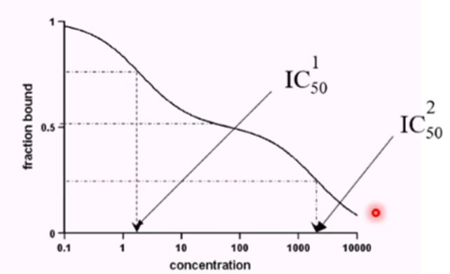
• Displacement curves can also show the presence of multiple binding sites 

  • E.g if there are 2 receptor sites to which the radiolabelled ligand binds with equal affinity, but which have different dissociation constants then they will be displaced at different conecntrations  

  • Can observe two humps in our displacement curve and we have to raed off 2 IC50 values (sometimes may not be well resolved if the Kd is similar) 

  • If we are still unsure of whether the displacement curve shows site heterogeneity then we can always do a hill plot analysis to determine this 

 

Cloned receptors

• If we clone receptors and express them in a given cell model, sometimes there will be G proteins that these cloned receptors couple to that they wouldn’t normally do  

• If this is the case, sometimes if we trigger a conformational change then we trigger other downstream effects → this can make our displacement curve shallower 

• Biological context of the experiment is important  

• Example: looking at beta receptors and looking for agonists often measured by the displacement of 125I cyanopondolol → Displacement curves showing single binding sites in cells lacking the G protein but show complex binding curves in cells which express the G protein