K65MMEI Oral Exam Preparation Flashcards

Vocabulary and concept flashcards covering Simplex method calculations, linear programming assumptions, graph theory algorithms, and project management principles based on the MMEI oral exam notes.

Operations Research

The use of mathematical methods to support decision-making by finding the best possible solution when resources are limited.

Typical models: linear programming, transportation, network, project management, inventory models

Describe the process of developing a mathematical model

1. Understand the real problem and goal

2. Identify variables

3. Set constraints

4. Create the objective function

5. Solve the model

6. Check the result

Compare parameters and variables in mathematical models

variables are unknown values that the model must find. Ex; x1=number of product A

Parameters are known fixed values from the problem. Ex; profit per unit, capacity

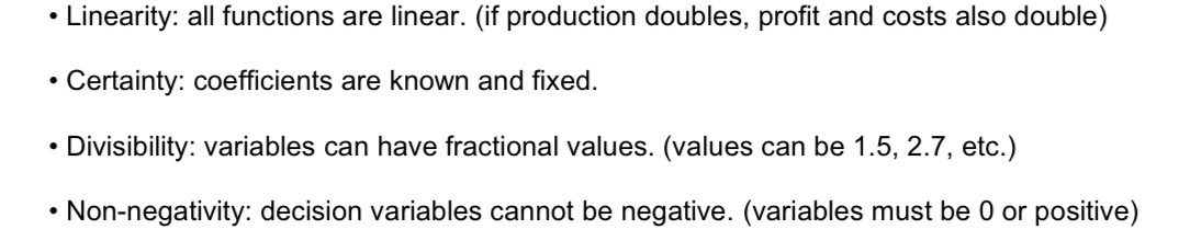
List at least three key assumptions in lp

Identify and describe the essential components of an LP model.

An LP model contains decision variables, an objective function, constraints, and non-negativity conditions.

Example: Max Z = 40x1 + 160x2, subject to resource constraints and x1, x2 >= 0.

Define constraints in LP and explain how they are represented.

Constraints are restrictions or limits in the problem.

They are written as linear inequalities or equations, for example 2x1 + 3x2 <= 100.

Describe the objective function in LP

The objective function is the model's goal.

It can be maximization, for example Max Z = 40x1 + 160x2, or minimization, for example Min C = 5x1 + 8x

Explain how to convert one type of objective in LP

A maximization problem can be converted to minimization by multiplying the objective function by -1.

Example: Max Z = 40x1 + 160x2 is equivalent to Min (-Z) = -40x1 - 160x

Difference between maximization and minimization in the simplex metho

The calculation idea is the same, but the optimality test has the opposite sign.

If the table uses zj - cj: for maximization the solution is optimal when all zj - cj >= 0; for minimization when all zj - cj <=0

Alternative Optimal Solution

Occurs when a problem has more than one best answer, indicated in a simplex table when another variable in the optimality test row has a value of $0$.

Degenerate Solution

A solution where at least one basic variable is equal to zero ($b = 0$ in a row of a basic variable in the simplex table).

Unbounded Solution

A case where the objective function can improve without limit, appearing when an entering variable can improve the objective but its column provides no valid leaving variable.

Infeasible Solution

A solution that does not follow the problem's rules; in simplex with artificial variables, it occurs when an artificial variable remains positive in the final solution.

How to determine the optimal solution graphically

1. Draw all constraints.

2. Find the feasible region.

3. Find all corner points.

4. Calculate the objective function at each corner point.

5. Choose the highest value for maximization or the lowest value for minimization.

Feasible Region

The area constructed by drawing all constraints that satisfies/follows all restrictions at the same time.

Redundancy

A situation where a constraint is unnecessary because it does not change the feasible region or the solution.

Parametric solution vector and basic solution.

A parametric solution vector shows the solution using parameters and gives all possible solutions.

• How many variables in a basic solution have non-zero values?

The number of non-zero variables is equal to the number of constraints.

• Define the basic solution in the simplex method.

The basic solution is a solution where basic variables have values and all non-basic variables are set to zer

B-inverse Matrix ($B^{-1}$)

The inverse of the basis matrix found in the slack variable columns ($s_1, s_2, s_3$) of a final simplex table; used to find new solutions by multiplying it by new Right-Hand Side (RHS) values.

LP model for production planning

Variables represent quantities of products to produce.

Typical objective: maximize profit or minimize production cost.

Typical constraints: machine time, labour, materials, demand, storage, budget

LP model for diet problems

Variables represent amounts of foods.

Typical objective: minimize total cost.

Typical constraints: minimum calories, proteins, vitamins, minerals, and maximum limits for fat, sugar, or salt.

LP model for cutting stock problems

Variables usually represent cutting patterns.

Typical objective: minimize waste or minimize the number of raw rolls/sheets used.

Typical constraints: required number of pieces of each size and material length/width limit

LP model for employee scheduling problems

Variables represent number of employees assigned to shifts or days.

Typical objective: minimize labour cost or number of workers.

Typical constraints: required workers per period, working hours, days off, and labour rule

Main components of the transportation model.

The main components are sources, destinations, supply, demand, transportation costs, and shipment variables xij.

If a transportation connection is unavailable, we remove that variable or put a very large cost M so it will not be

chosen.

Chinese Postman Problem

The goal of finding the shortest closed route that uses every edge at least once by duplicating shortest paths between paired odd-degree vertices to make the graph Eulerian.

1. Find all odd-degree vertices.

2. Pair them with minimum additional distance.

3. Duplicate the shortest paths between paired odd vertices.

4. The graph becomes Eulerian.

• Odd-degree vertex: a vertex with an odd number of incident edges.

• Eulerian circuit: a closed route that uses every edge exactly once.

Path vs. Cycle

A path starts at one vertex and ends at another; a cycle starts and ends at the same vertex.

Paths are used in shortest path and flow models. Cycles are important in routing problems, such as Traveling

Salesman Problem(TSP) or Chinese Postman.

Complete graph and chromatic number

A complete graph is a graph where every pair of vertices is connected by an edge.

For a complete graph with n vertices, the chromatic number is

Weighted graph.

A weighted graph has numerical values on its edges.

Weights can mean distance, cost, time, capacity, profit, risk, or length depending on the model

Chromatic number and map colouring

The chromatic number is the minimum number of colours needed so that adjacent vertices have different colours.

In scheduling, colours can represent time slots. Tasks connected by an edge cannot be in the same time slot.

In map colouring, neighbouring regions must have different colours.

Maximum Flow Problem.

The goal is to send the maximum possible flow from a source node to a sink node.

Nodes represent points in the network, edges represent possible routes, and capacities represent maximum allowed

flow on each edge.

Ford-Fulkerson algorithm.

1. Start with zero flow.

2. Find an augmenting path from source to sink.

3. Find the bottleneck capacity, the smallest residual capacity on that path.

4. Increase the flow by this bottleneck.

5. Update the residual graph.

6. Repeat until no augmenting path exists.

Key terms in flow networks

Augmenting path: a path from source to sink where additional flow can still be sent.

Residual graph: a graph showing remaining capacities and possible reverse flows.

Bottleneck capacity: the smallest residual capacity on an augmenting path.

Saturated edge: an edge on which the flow reaches its capacity. An augmenting path becomes saturated when at

least one edge on the path reaches its capacity.

Three key rules of feasible network flow.

• Capacity limits: flow on each edge cannot exceed its capacity.

• Flow conservation: for every intermediate node, inflow equals outflow.

• Source and sink rule: at the source, outflow - inflow equals the value of the flow; at the sink, inflow - outflow equals

the value of the flow.

Dijkstra Algorithm

Dijkstra algorithm finds the shortest paths from one starting node to all other nodes when edge weights are non-

negative.

1. Set the start distance to 0 and all others to infinity.

2. Choose the unvisited node with the smallest temporary distance.

3. Update distances to its neighbours.

4. Mark the node as visited.

5. Repeat until all needed nodes are visited.

In a graph, we mark distances near nodes. In an adjacency matrix, we read edge lengths from the matrix.

Minimum Spanning Tree (MST)

A spanning tree that connects all vertices ($n$) using $n - 1$ edges with the minimum total edge weight.

Prim vs. Kruskal Algorithms

Prim grows one tree from a vertex by adding the cheapest connected edge; Kruskal sorts all edges by weight and adds the cheapest ones while avoiding cycles.

Degree Centrality

Measures direct connections; normalized degree centrality is calculated as $\frac{\text{degree}}{n - 1}$.

Betweenness Centrality

Measures how often a node lies on shortest paths between other nodes; calculation involves checking if $d_{ij} = d_{ik} + d_{kj}$ for a node $k$.

Project Golden Triangle

The constraints of time, cost, and scope/quality in project management.

Activity-on-Arrow (AOA)

A project diagram method where activities are represented as arrows and nodes represent events.

Activity-on-Node (AON)

A project diagram method where activities are the nodes and arrows show dependencies.

Work Breakdown Structure (WBS)

A division of a project into smaller work packages and activities used before building the network in CPM.

Critical Path

The longest path in a project network which determines the total project duration.

Total Float (TF)

Calculated as $LS - ES$ or $LF - EF$.

Free Float (FF)

The minimum earliest start of successor activities minus the earliest finish of the current activity.

Dummy Activity

A fictive arc in a CPM graph with zero duration used to show logical dependencies.

Waterfall vs. Agile

Waterfall is sequential and best for stable requirements; Agile is iterative and flexible for changing requirements.

Excentric Node

The starting node in an oriented CPM network graph.

Concentric Node

The ending node in an oriented CPM network graph.