AP STATS Important things to Memorize

describing a display of univariate data

SOCS:

• shape (include skew or roughly symmetric, and modality)

• Outliers/unusual features (include gaps and/or outliers)

• center (mean if symmetric, median if skew)

• spread (standard deviation if symmetric, IQR if skew)

Make sure you choose most powerful center and spread correctly for the given shape.

When making quantitative displays (histograms, boxplots, stemplots)...

you must include:

-labels and quantities on both axes

-key for a stemplot

If you are asked to compare two distributions

use words like: "greater than," "less than" or "about the same as" ... it's not enough to just list SOCS for both if you're asked to compare

interpreting standard deviation

The average distance of each [description of the data] is from the mean of [xbar] is [Sx].

Example: The average distance of each person's metabolic rate from the mean of 1600 is 189 calories per 24-hour period.

interpreting a z-score

The [piece of data] is ________ standard deviations above/below the mean.

If a z score is 1.45, that means the value is 1.45 standard deviations above the mean. Shape does not have to be normal to calculate a z-score. You can standardize any data set.

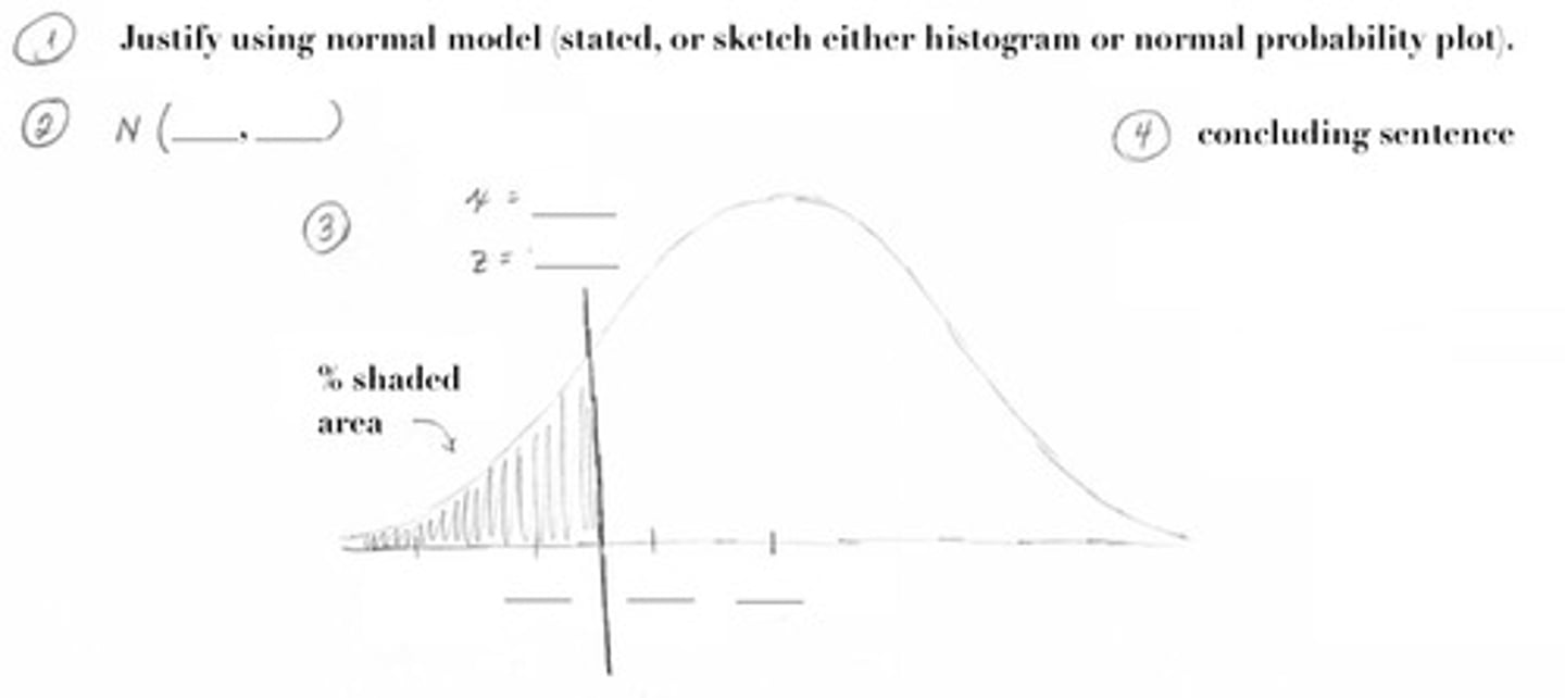
justify using a normal distribution by...

• stating you were told data were roughly normal

• providing a reasonably accurately sketched histogram

• providing a reasonably accurately sketched normal probability plot (last option in STAT PLOT menu). A linear probability plot implies distribution is normal.

labeling a normal distribution

mean goes in the middle; standard deviation is the scale to go by; go three up and then three down

describing a scatter plot

DOFS:

• direction (positive or negative)

• unusual stuff (any potential outliers that would affect the LSRL if removed)

• form (roughly linear or curved)

• linear strength of that shape (strong, moderately strong, moderate, fairly weak, very weak,etc. supported by the correlation coefficient-- "r")

interpreting slope

for every additional 1 [explanatory variable], the predicted [response variable] increases/decrease by [slope].

interpreting r (correlation coefficient)

r: correlation coefficient measures LINEAR strength of the model

-1 < r < 1

-1 is strong negative linear association

1 is strong positive linear association

closer to 0 implies weak or no association

correlation does not imply causation! causation can be concluded if an experiment was conducted.

interpreting r-squared (coefficient of determination)

About ________ % of the variability in (response variable, because, ewww, we dont talk about our x's) is explained by the model's linear relationship to (explanatory variable).

setting up a simulation

• Describe action to be repeated.

• Using a random number generator [or table], use digits ______ through ______ to represent __________. [If using a table, specify whether any digits need to be ignored.]

*You can also use equal size slips of paper in a hat... instead of random digit table

• Describe how to put the repeated actions into a trial.

• Allow or don't allow for repeated digits. Specify what you will be recording.

analyzing the results of the simulation

Write out assumptions:

• include assumption of exactly what measured trait is independent of the next

• include any other stated assumptions used

Write out anaylsis:

• Based on ____ random trials, I (would/not) expect to find ______ (results) in more than ______ (determined probability). _ (state if unusual or not).

justifying independence in Probability

P(A) x P(B) = P(A and B)

The products must equal the "both"/intersection

a "go-to" example of disjoint/mutually exclusive events NEVER being independent

getting an A or a B in stats class:

There's no overlap... can't get both an A and a B at the same time.

Once I get an A, it reduces my chance of getting a B to 0.

finding P (at least....) or P (at most...) when binomial

write out first two terms and last before using binomcdf to help you see which way you will calculate; 1 - binomcdf for greater than scenarios

justifying use of a normal curve to approximate a binomial histogram

np = _____ and n(1 - p) = _____, both at least 10

describing a distribution

state whether normal, binomial, or t

if normal, include mu and sigma

if binomial, include n and p

if t, include mu, sample standard deviation, and degrees of freedom

conditions for using inference for the distribution of ONE sample proportion

• RANDOM: Assume/given a random sample

• NORMAL: np = _______ and n(1 - p) = _______, both at least 10

• INDEPENDENT: Assume a population is at least 10 times your sample size

conditions for using inference for the distribution of ONE sample mean

• RANDOM: Assume/given

• NORMAL: n > 30, so sample is big enough

OR if n < 30, but we're told the original population is normal OR n < 30 distribution is roughly normal, as evidence of (show either a histogram or dotplot or a roughly linear normal probability plot)

• INDEPENDENT: Assume a population is at least 10 times your sample size

interpreting a confidence LEVEL

If many similar samples were taken, _____% of them would result in intervals that contain the true mean/proportion.

interpreting a confidence INTERVAL

We are ____ % confident the interval from ___ to ___ captures the true mean/proportion of ________________ (provide context)

* 95% does NOT mean that there is a 95% chance that the true _____ is in the given interval or not: the true mean either IS or IS NOT in that interval

interpreting a p-value

If _________________ (null) were true, _____% (p-value) of similar samples would have results of at least/at most _____________________ (provide context for the shaded region in your normal curve).

drawing a conclusion from a low p-value (improbable results if null is true)

Given a low p-value of ______, we reject the null.

We have sufficient evidence at alpha = ___ to conclude Ha (in context)

[The difference we observed is likely due to something besides sampling variability]

drawing a conclusion from a high p-value

Given a high p-value of _______, we fail to reject the null.

We have insufficient evidence at alpha = ___ to conclude Ha (in context)

[The difference we observed is likely due simply to sampling variability.]

assumptions and conditions for chi-square test for ONE group, MULTIPLE variables (independence) : Example would be recording speed and agefor 200 drivers to see if those traits are independent.

• EXPECTED counts all greater than 5.

• random and/or representative samples

assumptions and conditions for chi-square test for TWO or more groups, one trait measured (homogeneity): Example would be recording speeds for 100 young drivers and then for 100 older drivers to see if the distribution of speeds is different from one age to the next.

• EXPECTED counts all greater than 5.

• random and/or representative samples

assumptions and conditions for linear regression test

LINER:

• Scatterplot is roughly linear.

• Independence (Assume a population is at least 10 times your sample size for each sample)

• histogram of residuals is roughly normal (or normal probability plot is roughly linear).

• Equal variance: Residuals are evenly scattered, randomly spaced

•Random sample