econ m2

Demand Increases (up arrow), Supply Increases (up arrow)

Effect on Price (P): Ambiguous (Depends on shift size)

Effect on Quantity (Q): Increases (Both want more sold)

Demand decreases (down arrow), Supply decreases (down arrow)

Effect on Price (P): Ambiguous (Depends on shift size)

Effect on Quantity (Q): Decreases (Both want less sold)

Demand Increases (up arrow), Supply Decreases (down arrow)

Effect on Price (P): Increases (High demand, low supply)

Effect on Quantity (Q): Ambiguous (Depends on shift size)

Demand Decreases (down arrow), Supply Increases (up arrow)

Effect on Price (P): Decreases (Low demand, high supply)

Effect on Quantity (Q): Ambiguous (Depends on shift size)

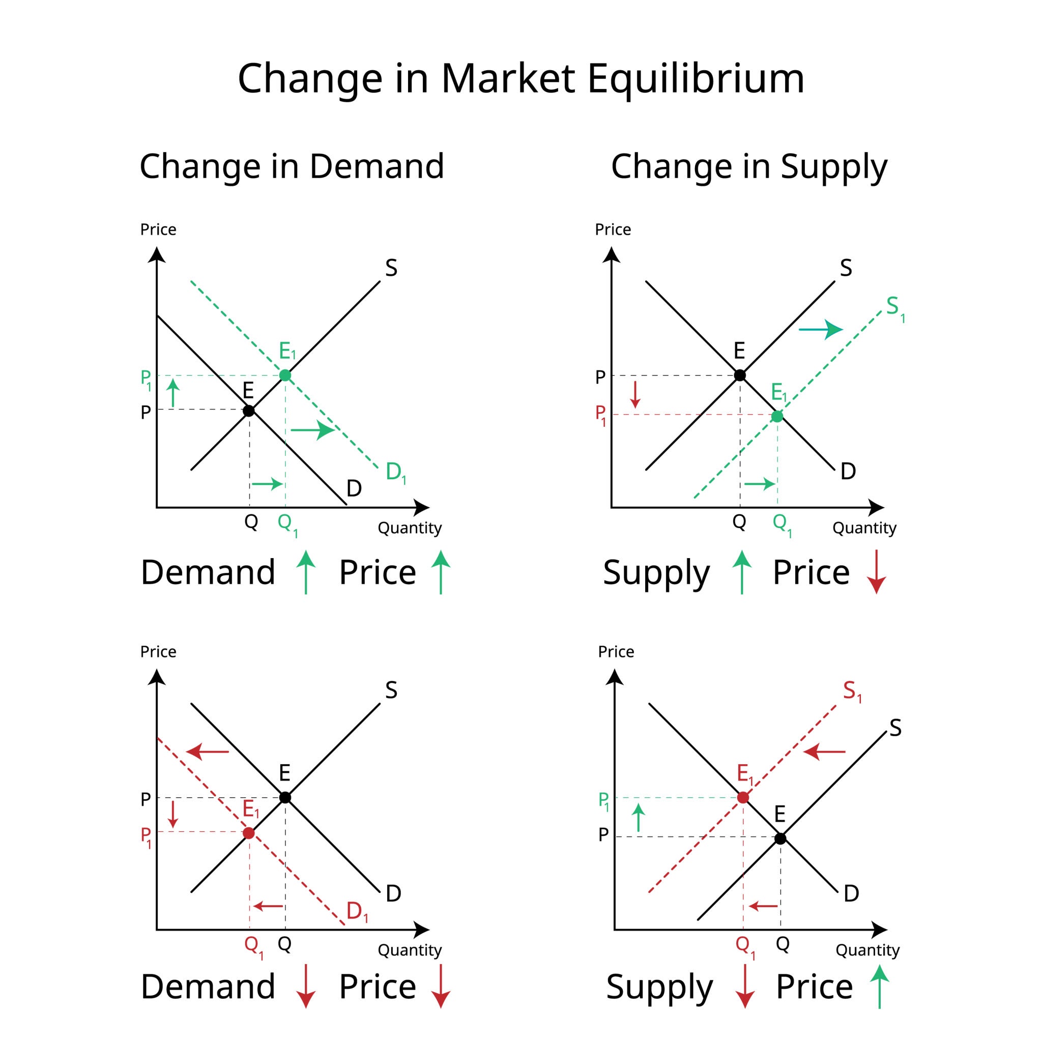
If people want more product (D arrow up) the price and quantity goes…

Price goes UP

Quantity goes UP

If the product becomes harder to make (Supply down arrow) price and quantity goes…

Price goes UP

Quantity goes DOWN

For Price: Since both of those shifts push the price up (UP + UP) what happens….

Price definitely Increases

For Quantity: The demand wants it up, Supply want it down (UP + DOWN) what happens…

The Quantity is Ambigous

Ex. Demand Increases significantly, Supply only a little bit. what happeneds

The Up from the demand shift is much stronger than the down from the supply shift. The Price increases and Quantity increases.

What is a Price Ceiling?

A Price Ceiling is a government imposed limit on how high a Price can go. It must be set below the equilibrium price. Ex. Rent Control

Impact on Market: Shortage (Quantity demand > Quantity supply)

What is a Price Floor?

A Price Floor is a government-imposed limit on how low a Price can go. Ex. Minimum wage. Must be set above the equilibrium price.

Impact on Market: Surplus ( Quantity supply > Quantity demand)

What is DWL (Dead Weight Loss)?

It represents missed opportunities. Its the value of trades that should have happened but didn’t.

If the price is capped too low (ceiling), demand exceeds supply. Sellers can’t raise the price, so they extract value elsewhere:

Key Fees: The rent is $500, but its $2,000 to get the key.

Bribes: Sliding a $50 bill to a waiter to get a table in a Price controlled restaurant.

Price Ceiling (D > S): Sellers have more customers than goods. They don’t need to be nice or provide a good product. Ex…

Ex. A lard lord stops fixing the heater because there is a line of people waiting to rent the apartment regardless of its condition (Quality drops)

Price Floor (S > D): Sellers have too much product and not enough buyers. They can't lower the price, so they compete on "frills." Ex…

Ex. Airlines in the 1970s had regulated high fares. Since they couldn't lower prices, they competed with steak dinners and luxury service.

Why this doesn’t really work: Most travelers would rather have a $200 cheap flight than a $500 luxury flight, but the floor forces them to pay for quality they don't actually value.

When the minimum wage is set above the market equilibrium for low-skilled labor:

Surplus (Unemployment): More people want to work at better-paying jobs than the jobs available.

Disemployment: Companies reduce the number of employees or automate tasks (Self-checkout kiosks).

Benefit Offsets: If a boss is forced to pay more in cash, they might take away "hidden" pay like free shift meals, 401k matching, or flexible scheduling.

If the Supply of Labor is Inelastic (Steep), workers don't have many other options. They will keep looking for jobs even if the wage changes.

In this case, a minimum wage increase causes a smaller increase in unemployment because workers aren't flooding into the market from elsewhere they were already there.

The case against minimum wage…

It hurts the most vulnerable: It "prices out" workers whose skills aren't yet worth the legal minimum, preventing them from getting the "first rung" of experience.

Hidden Costs: It leads to worse working conditions and fewer fringe benefits.

Inefficiency: It creates DWL by preventing mutually beneficial low-wage contracts.

The case for minimum wage:

Monopsony Power: In the real world, employers often have more bargaining power than workers. A minimum wage "levels the playing field."

Increased Productivity: Higher wages can lead to "Efficiency Wages," where workers work harder and quit less often because they value their job more.

Macro-Stimulus: Low-income workers spend almost every dollar they earn, which can boost local demand for goods and services.

The Opposite curve rule.

To predict how much P* and Q* will change:

If Demand shifts, look at the Supply Curve.

If supply shifts, look at the slope of the Demand curve.

Because the shift forces you to "slide" along the other curve to find the new equilibrium. The other curve is the "track" you are stuck on.

The Inelastic Steep Curve Scenario

Think of an inelastic curve as Stubborn.

If Supply shifts along Inelastic Demand: Consumers need the product (like insulin or gasoline). They will pay almost any price to get it.

The Result: P* swings wildly, but Q* barely moves.

The Elastic Flat Curve Scenario

Think of an elastic curve as Sensitive.

If Supply shifts along Elastic Demand: If the price goes up even a little, consumers stop buying.

The Result: Q* drops significantly, but P* can't rise much because the sellers would lose all their customers.

Slope is about absolute change.

Slope is constant on a straight line. If you move one inch on the graph, the slope value is the same.

Elasticity is about percent change.

Elasticity changes as you move along the line.

A $1 increase on a $2 item is a 50% increase (Huge deal!).

A $1 increase on a $100 item is a 1% increase (Who cares?).

Even if the "slope" is the same, the responsiveness (elasticity) is much higher when prices are low and quantities are high.

The Time Factor: Short Run

Short Run = Inelastic: If gas prices double today, you still have to drive to work tomorrow. You are "stuck."

The Time Factor: Long Run

Long Run = Elastic: Over two years, you can buy a fuel-efficient car, move closer to work, or start carpooling. You become more responsive over time.

The burden of a tax falls most heavily on the party that is less elastic (more stubborn/less flexible).

Elasticity = Escape: If you are elastic, you can "run away" from the tax by changing your behavior (buying something else or producing something else).

Inelasticity = Trap: If you are inelastic, you are "trapped" in the market and will end up paying the tax regardless of who the law says is responsible.

Relative Elasticity Scenarios

Consumers are more elastic (D is flatter than S): Consumers find substitutes. Producers are stuck with the product and must lower their prices to keep selling. Producers pay more.

Producers are more elastic (S is flatter than D): Firms move their factories or stop making the good. Consumers need the good and will pay a higher price. Consumers pay more.

Visualizing the Tax: The Wedge Method

Imagine a wedge being driven between the price the buyer pays (Pb) and the price the seller receives (Ps).

How to read the graph:

The Wedge: The height of the wedge is the Tax per unit.

1. P^b (Price Buyers pay): This is the top of the wedge, where it hits the Demand curve.

2. P^s (Price Sellers get): This is the bottom of the wedge, where it hits the Supply curve.

3. Consumer Burden: The distance from the old Equilibrium (P*) up to P^b.

4. Producer Burden: The distance from the old Equilibrium (P*) down to P^s.

Deadweight Loss (DWL) and Government Revenue

A tax creates a "gap" in the market that prevents mutually beneficial trades from happening.

Government Revenue: This is the rectangle formed by the Tax x New Quantity (Qtax). This is money transferred from citizens to the state.

Deadweight Loss (DWL): This is the "Yellow Triangle" to the right of the tax wedge. It represents the trades that would have happened at the original equilibrium but were "killed" by the tax.

Key Insight: The more elastic the curves are, the larger the DWL will be. Why? Because elastic people change their behavior a lot in response to the tax, meaning more trades are canceled.

Why the "Statutory" Burden Doesn't Matter

If the government passes a law saying "Sellers must pay a $1 tax on every apple," the Supply curve shifts up by $1. If they say "Buyers must pay the $1 tax," the Demand curve shifts down by $1.

If you draw both, you will find that the final price paid by consumers and the final price kept by sellers is exactly the same in both scenarios. The market cares about the total cost, not whose hand physically hands the money to the IRS.

Practice: Demand is very elastic (rich people can just buy a beach house or a private jet instead).

Demand is very elastic (rich people can just buy a beach house or a private jet instead).

Supply is inelastic (yacht builders have specialized factories and workers that can't easily switch to making something else).

Fixed Inputs

These are resources that cannot be changed quickly, regardless of how much output you want to produce.

• The Constraint: Even if you want to double your production tomorrow, you are "stuck" with the current amount of these inputs.

• Examples: A factory building, a specialized pizza oven, or a 10-acre farm. You can’t just "manifest" a second factory overnight.

Variable Inputs

These are resources that can be changed easily and quickly to increase or decrease production.

• The Flexibility: If business picks up on a Friday night, you can pull this lever immediately.

• Examples: Hourly labor, raw materials (flour, steel, electricity), and packaging.

Short Run vs. Long Run

In economics, these aren't specific time periods (like "six months"); they are defined by your inputs.

• The Short Run: A period of time where at least one input is fixed. (Usually, the building or heavy machinery is fixed, while labor is variable).

• The Long Run: A period of time long enough that all inputs become variable. Given enough time, you can build a new factory, buy 50 more ovens, or sell your land.

Key Takeaway: In the short run, if you want to produce more, your only option is to hire more workers (variable input) to work within your existing building (fixed input).

Why labor is the classic Variable Input

Labor = Variable: You can ask employees to work overtime, hire a temp, or send people home early if it's slow.

Capital/Land = Fixed: You are usually signed into a lease or waiting for equipment to be delivered and installed.

The crowding effect

Because you have a fixed input (like a small kitchen) and a variable input (workers), you eventually run into a problem. If you keep adding workers to that one small kitchen, they start bumping into each other. This leads to Diminishing Marginal Product.

Ex. Food Truck

• Fixed Input: The Truck itself. (You can't make it bigger during the lunch rush).

• Variable Input: The staff and the taco shells.

If the line is down the block, the owner can't buy a new truck instantly, but they can call a friend to come help for two hours.

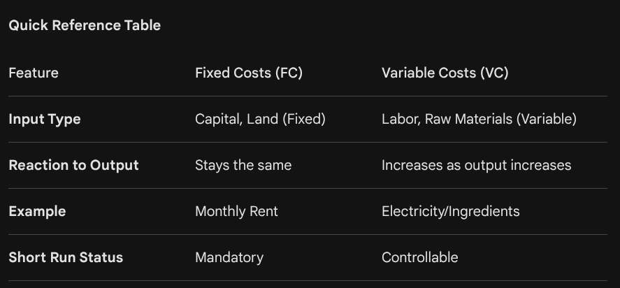
Fixed Inputs and Fixed Costs

Fixed Costs are expenses that do not change with the level of output. Fixed inputs are resources that can not be easily increased or decreased in a short period.

Input: Physical capital (factories, heavy machinery, equipment)

Cost: Rent, Insurance, property taxes or interest

In the short run these are sunk. You are committed to them regardless of how much you sell.

Variable Inputs and Variable Costs

Variable costs change directly with the volume of production. If you want to produce more, you need more inputs. These correspond to variable inputs

Inputs: Labor (hourly workers) and raw materials (flour for a bakery, steel for a car)

Costs: Wages, electricity used for production, and the cost of ingredients.

Key: These costs start at zero when production is zero and rise as output increases.

Total Cost Equation

TC = FC + VC

As you increase production, the TC curve takes its shape from the VC curve, but it starts higher up on the y axis because of the FC.

Diminishing Marginal Returns x Variable Cost

Early Stages: Adding more variable inputs (workers) to a fixed input (a kitchen) might make you more efficient (specialization), so costs rise slowly.

Later Stages: Eventually, adding more workers to that same fixed kitchen leads to crowding. Each new worker adds less to total output than the previous one, causing your variable costs to spike.

In the long run, there are no fixed costs. A company can build a second factory or move to a smaller office. Therefore, all fixed inputs eventually become variable inputs given enough time.

Total and Average Cost

Primary formula ATC = TC/q

To find Total Cost: TC = ATC x q

To find Quantity q = TC/ATC

Breaking down the average

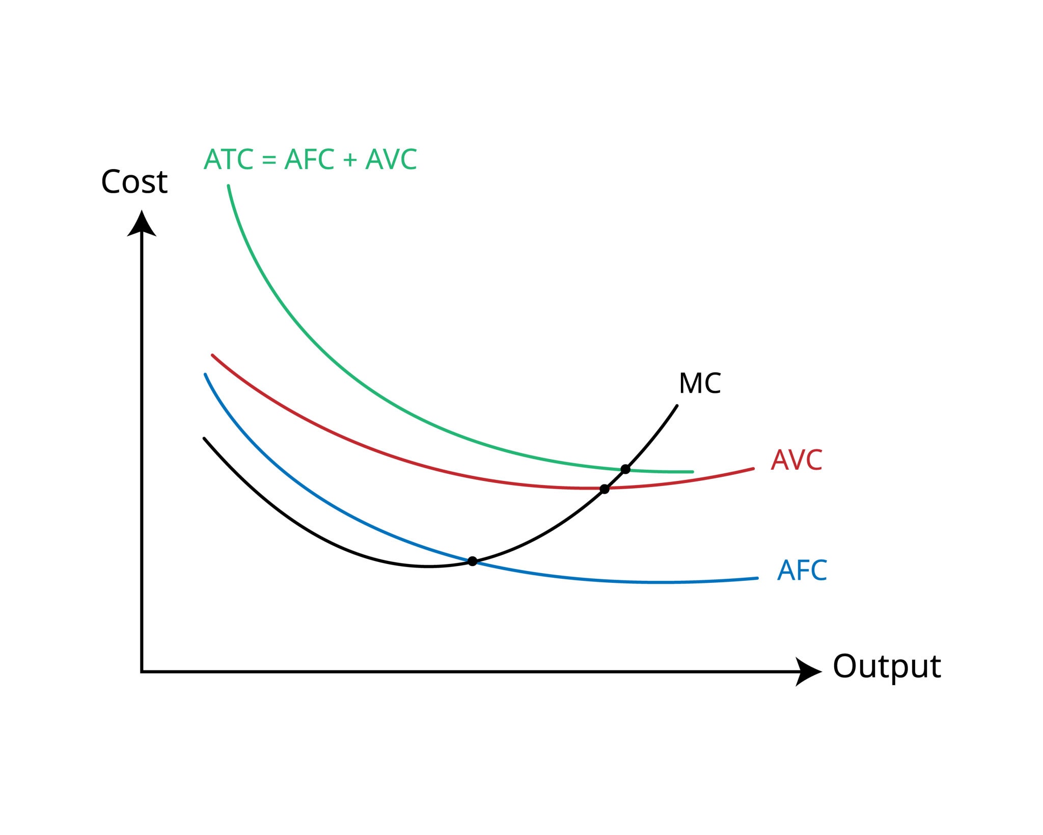
Average Total Cost: ATC = AFC + AVC

If a pizza shop has an AFC of $2.00 (rent/ovens) and an AVC of $5.00 (dough/cheese), the ATC per pizza is $7.00.

Visualizing the Curves

AFC (The "Slide"): This curve always slopes downward and never touches the x-axis. It gets smaller and smaller as q increases.

AVC (The "U-Shape"): It drops initially due to efficiency, then rises because of diminishing returns.

ATC (The "U-Shape"): This sits above the AVC. The vertical distance between the ATC and AVC curves is the AFC. Notice that as production increases, the ATC and AVC curves get closer together (because AFC is shrinking).

Fixed Cost Spreading

Fixed-cost spreading occurs when you increase output (q), causing the "burden" of your fixed costs (TFC) to be shared across more units.

Scenario A: You pay $1,000 in rent and make 1 widget. Your fixed cost per unit is $1,000.

Scenario B: You pay $1,000 in rent and make 1,000 widgets. Your fixed cost per unit is now only $1.

This is why big factories love high-volume production; they "spread the overhead" so thin that the fixed cost per item becomes negligible.