Transport | All 2

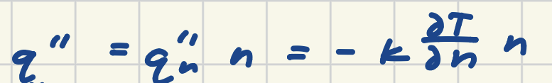
qn” = heat flux in a direction n, which is NORMAL to an isotherm! n = unit vector in that direction;

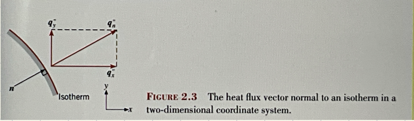
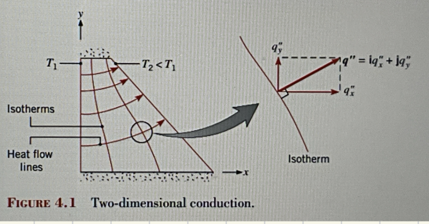
Figure 4.3: 2-D conduction

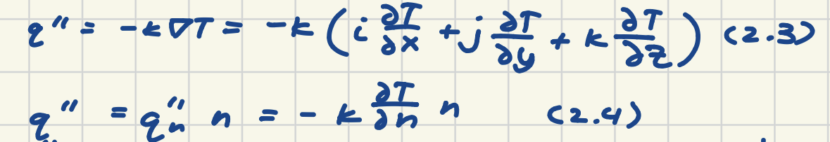
heat transfer is sustained ny a temperature gradient ALONG n (n = vector perpendicular to the isotherm, qn" = perpendicular to the isotherm). Note that also the heat flux vector ca be resolved into components, such that in cartesian coorfinates, the general expression for q” is Eq. 2.3 or 2.4. q” = qn” * n!!! (Eq. 2.3)

heat flow line

adiabats; since heat flow lines are BY DEF in the direction of heat flow, no heat can be conducted across a heat flow line, and they are sometimes referred to as adiabats!

tangent

“tangent to a direction” generally means aligned with (or pointing along) that direction, but it’s more precise than just “along.”!!!!!!!!

more on adiabats/heat flow lines

since no heat crosses a heat flow line, each line acts like a surface across which heat doesn’t flow - like an adiabatic barrier (why heat flow lines are referred to as adiabats!)

perpendicular to heat flow lines

isotherms; represent constant temperature surfaces

conduction analysis

1.) if can determine the temperature distribution in the medium, which for the present problem, necessitates determining T(x,y). To do this, we solve the appropriate form of the heat equation (by using Fourier’s Law) (methods to solve heat equation include analytical, graphical, and numerical [such as FINITE-DIFFERENCE, finite-element, or boundary element] approaches). 2.) if we can solve for T(x,y), it is easy to satisfy the second objective (which is to determine the heat flux components qx” and qy” by applying the rate law equations (Fourier’s Law in 2-D)

finite-difference equations

node equations

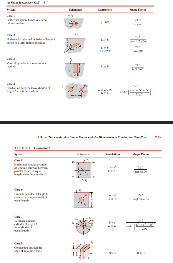
conduction shape factor and dimensionless heat rate

In general, finding analytical solutions to the two- or three-dimensional heat equation is time-consuming and, in many cases, not possible. Therefore, a different approach is often taken. For example, in many instances, two- or three-dimensional conduction problems may be rapidly solved by utilizing EXISTING solutions to the heat diffusion equation. These solutions are reported in terms of a shape factor S or a steady-state dimensionless conduction heat rate, q*ss. The shape factor is defined such that

q = Sk ∆T1-2

∆T = temperature difference between boundaries, for example shown in Fig. 4.2. It also follows that a 2-D conduction resistance may be expressed as

Rt,cond2-D = 1/(Sk).

Shape factors have been obtained analytically for numerous two- and three-dimensional systems, and results are summarized in Table 4.1 for some common configurations. Results are also available for other configurations [6–9]. In cases 1 through 8 and case 11, twodimensional conduction is presumed to occur between the boundaries that are maintained at uniform temperatures, with ∆T1−2 = T1 − T2.

Some shape factor / dimensionless conduction heat rates for selected systems (Table 4.1)

nodal analysis can be scaled in industry via existing software options

Ex. Ansys Fluent, COMSOL, Open FOAM. YOUR ROLE then becomes: specifying geometry, stating boundary conditions, and MESH REFINING

PYTHON versus ANSYS for solving 2D conduction, nodal analysis, aka ways to estimate 2d conduction and temperature gradients

Python is free and would useful for personal projects and simple geometries. Fluent is costly and is useful for modelling complex geometries and FINER MESHES.