1725 Principles of Digital Radiography

Digital Radiographic Image Sampling

• 2 steps in image processing

  • Preprocessing: Takes place in the computer where the algorithms determine the image histogram

  • Postprocessing: Done by the technologist through various user functions

The Image Histogram

• Data recognition program searches for anatomy recorded on the imaging plate by

  • Finding collimation edges

  • Eliminating scatter outside the collimation

• Information within the collimated area is the signal used for image data

  • This is the source for a vendor-specific exposure data indicator

• Failure to find the collimation edges can result in incorrect data collection

  • Images may be too bright or too dark

• Equally important is centering anatomy to the center of the imaging plate

  • Ensures that appropriate recorded intensities are located

  • Failure to do so could result in an image that is too bright or dark

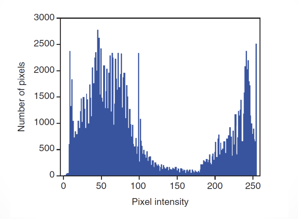
Histogram

• A graphical representation of exposure values collected from the imaging plate

  • Horizontal axis - tone values

  • Vertical axis - number of pixels in each tone

  • Values on one end represent the black areas (greater acquired signals)

  • Tones vary toward the opposite end and get brighter and the middle area is the medium tones

  • The extreme opposite end represents the white tones (no acquired signals)

Histogram Formation

• IR is scanned

• Image location and orientation are determined

• Size of the signal is determined

• Value is placed on each pixel

• A histogram is generated from the image data

Low energy (kVp) gives

A wider histogram

High energy (kVp) gives

A narrow histogram

Histogram shows

• The distribution of pixel values for any given exposure

• For example:

  • Pixels have values of 1,2,3, and 4 for a specific exposure

  • Histogram shows the frequency of each of those values and actual number of values

  • Histogram sets the minimum (S1) and maximum (S2) “useful” pixel values

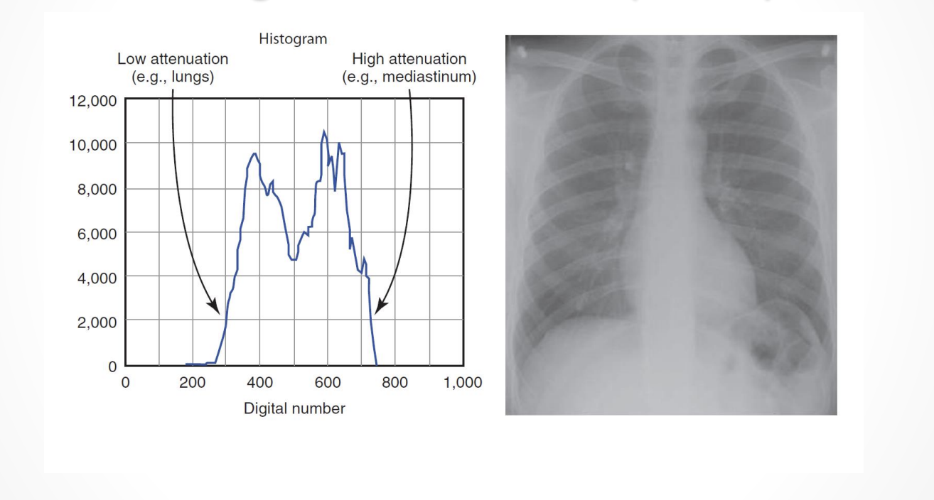
Histogram Analysis

• Analysis is complex

• Shape of the histogram stays fairly constant for each part exposed (anatomy specific)

• For example: Shape of histogram for a chest radiograph on a large adult patient looks different from a knee histogram generated from a pediatric knee exam

• Choosing the correct anatomic region on the menu before exposing the patient is essential

• Raw data used to form the histogram are compared with a “normal” histogram of the same body part by the computer

• Image correction takes place at this time

Digital Radiography Image Sampling

• Nyquist Theorem

• Aliasing

• Automatic Rescaling

• Look-up Table

The Nyquist Theorem

• The theorem states that when sampling a signal, the sampling frequency must be greater than twice the bandwidth of the input signal so that the reconstruction of the original image will be as close to the original signal as possible

  • At least twice the number of pixels needed to form the image must be sampled

  • If too few pixels are sampled, the result is a lack of resolution

  • Oversampling does not result in additional useful information

During image acquisition, energy conversion allow for signal loss. Conversions include

• X-rays to light to electrical signal (indirect capture)

• X-rays to electrical signal (direct capture)

• The indirect method of image acquisition has the highest potential for loss of signal

The PSP plates, The longer the electrons are stored, the more energy they lose

• When laser stimulates electrons, some lower energy electrons escape the active layer

• If enough energy was lost, some lower energy electrons are not stimulated enough to escape, and information is lost

• All manufacturers suggest that imaging plates be read as soon as possible to avoid this loss

Aliasing

• Occurs in digital imaging when:

  • Spatial frequency is greater than the Nyquist frequency

  • Sampling occurs less than twice per cycle

    • Information is lost

    • Fluctuating signal is produced

  • Also known as foldover or biasing

  • Causes mirroring of the signal at ¼ the frequency

  • A wraparound image is produced, and the image appears as two superimposed images slightly out of alignment

Aliasing Results in a moire effect

• The same effect can occur with grid errors

• When a sampled frequency is exactly at the Nyquist frequency, often a zero amplitude signal will result

  • Termed the critical frequency

  • Results from frequency phase shifts, causing aliasing of the signal

Automatic Rescaling

• Occurs when exposure is greater than or less than what is needed to produce an image

  • Images are produced that have uniform brightness and contrast regardless of the amount of exposure

Problems occur with rescaling

• Too little exposure results in quantum mottle

• Too much exposure results in a loss of contrast and loss of distinct edges because of detector saturation (This is very extreme)

• Rescaling is no substitute for appropriate technical factors

• Danger exists of using higher than necessary mAs values because doses will “creep” up over time

• To combat dose creep RTs should use standardized technique charts

  • Charts should be validated by radiologists to ensure an acceptable SNR

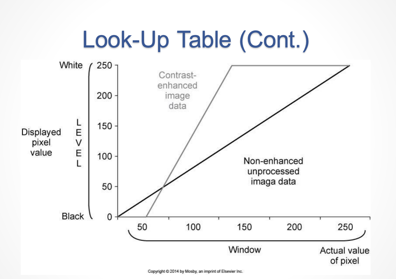
Look-Up Table

• Defined as a histogram of the luminance values derived during image acquisition

• Used as a reference

  • To evaluate the raw information

  • Correct the luminance values

• Is a mapping function:

  • All pixels are changed to a new grey value

  • Image will have appropriate appearance in brightness and contrast

• Provided for every anatomic part

Look-Up Tables can be graphed as follows:

• Plotting the original values ranging from 0 to 255 on the horizontal axis

• Plotting new values, also ranging from 0 to 255 on the vertical axis

• Contrast can be increased or decreased by changing the slope of the graph

• Brightness can be increased or decreased by moving the line up or down the y-axis