graph explanations for exams

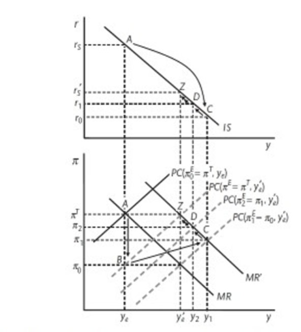
Positive permanent supply shock

Period 0: The supply shock stems from a shift in WS (WS-PS is not shown). Start at A, expected inflation is on target when the economy is at equilibrium output. The permanent positive S shock reflects e.g. reduced unemployment benefits, which would reduce worker bargaining power. This entails a shift down (rightwards) of WS: WS shifts right along the PS curve (assumed horizontal). Price markups are now too high, so firms reduce price inflation to restore markups. Similar permanent positive S shock effects would be felt from an upwards shift of the PS curve (increased product market competition or a rise in technical progress that boosts productivity). The WS shift boosts equilibrium employment and output. Assume that this shock occurs in period 0, before policy or expectations have a chance to react. Initially, actual output is well below equilibrium output 𝑦′𝑒, so there is a negative output gap. The PC shifts down, initially reflecting only this equilibrium output change; adaptive inflation expectations remain at 𝜋𝑇. (Highest dashed PC.) Actual output has not yet altered so the economy moves to B, on the new PC. The PC then shifts to reflect the lower inflation at B (𝜋0). The CB knows the shock is permanent, so MR shifts out, to MR’, to capture the fact the CB now wants to achieve 𝜋𝑇 at 𝑦′𝑒 rather than 𝑦𝑒. Given that the fall in inflation shifts the PC out / right to PC(𝜋𝐸1=𝜋0,𝑦𝑒) (furthest right), the CB chooses the interest rate corresponding to that PC’s intersection with MR’, choosing real interest rate 𝑟0. This interest rate is below the equilibrium rate, so output is higher than equilibrium output. Inflation starts rising but is still below target level.

Period 1: The PC adjusts to the new inflation rate, and the CB responds to this (forecast of) higher inflation by raising interest rates.

Period 2& onwards: Gradually inflation and real interest rates rise, and output falls, until equilibrium is achieved at Z.

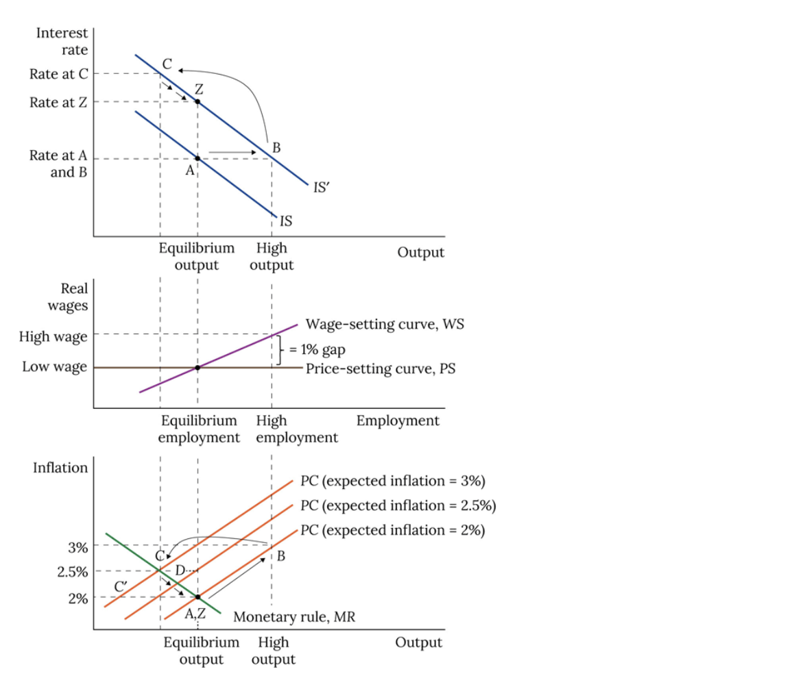
positive permanent demand shock

What happens immediately:

• IS curve shifts right (higher demand)

• Output ↑

• Employment ↑

• Unemployment ↓

Labour market effect:

• Tight labour market creates a 1% bargaining gap

• Workers demand:

  • 2% to compensate for last inflation

  • +1% extra due to stronger labour market

• Wages rise 3%

• Firms raise prices 3%

• Inflation rises to 3%

Graph movement:

• Move along Phillips Curve (expected inflation still 2%)

• Economy moves from A → B

next period Now:

• Expected inflation becomes 3% (higher wages become embedded in expectations of wage setters. for the next wage setting round, relevant PC facing the CB is new PC

• Phillips Curve shifts up to:

  • PC (expected inflation = 3%)

Central bank reaction:

• Does not want:

  • High inflation

  • Or a deep recession

• Chooses balanced response on MR curve

• Raises interest rates

Effects:

• Higher interest rate ↓ investment

• Aggregate demand ↓

• Output falls toward potential

• Economy moves to Point C

Next period

• new PC 2.5%.

bank keeps moving economy along MR curve and lowering rates until we reach target inflation and equilibrium output at new higher rates.

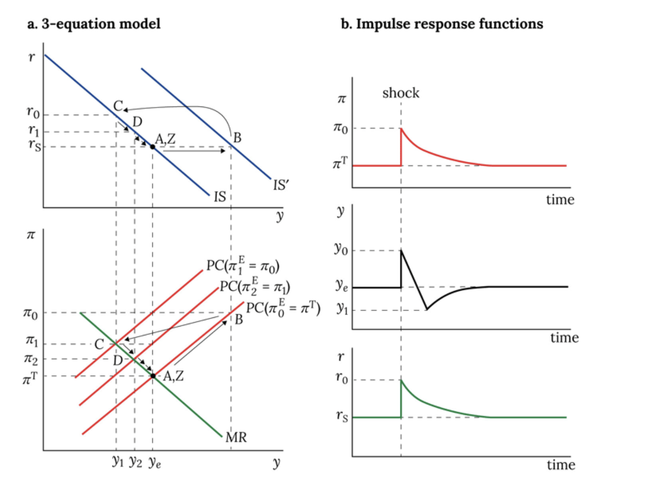
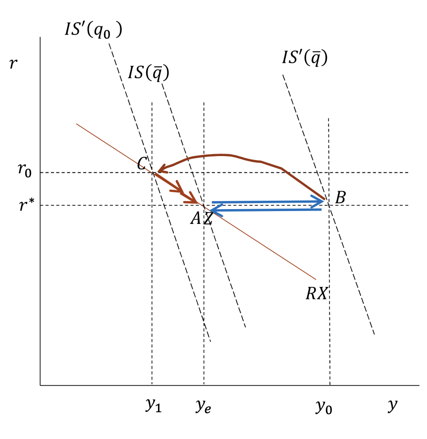
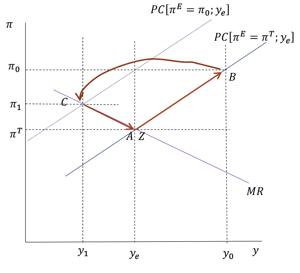
positive temporary demand shock

• IS shifts and stays at IS’ for one period

• the economy shifts from initial point A to point B

  The CB forecasts the PC for period 1, which is PC The CB expects that IS’ returns to IS at the beginning of period 1, and thus sets its interest

  rate on the basis of IS. The CB chooses 𝑟0 with the aim of achieving 𝑦1 and π1 in period 1.

  End of period 0 values: 𝜋0, 𝑦0, 𝑟0

  Period 1:

  The higher 𝑟0 reduces π, and 𝑦 goes below equilibrium 𝑦𝑒

  The CB forecasts PC for period 2 to be PC (𝜋2

  𝐸 = 𝜋1), so now, the best response is D; To

  achieve this, 𝑟0 is reduced to 𝑟 1.

  End of period 1 values: 𝜋1, 𝑦1, 𝑟 1

  Period 2 onwards:

  The economy moves to point D as demand increases as a result of lower 𝑟.

  The same process repeats and 𝑟 is gradually reduced until the economy reaches its

  equilibrium Z, given by π𝑇

  , 𝑦𝑒 and 𝑟 𝑆.

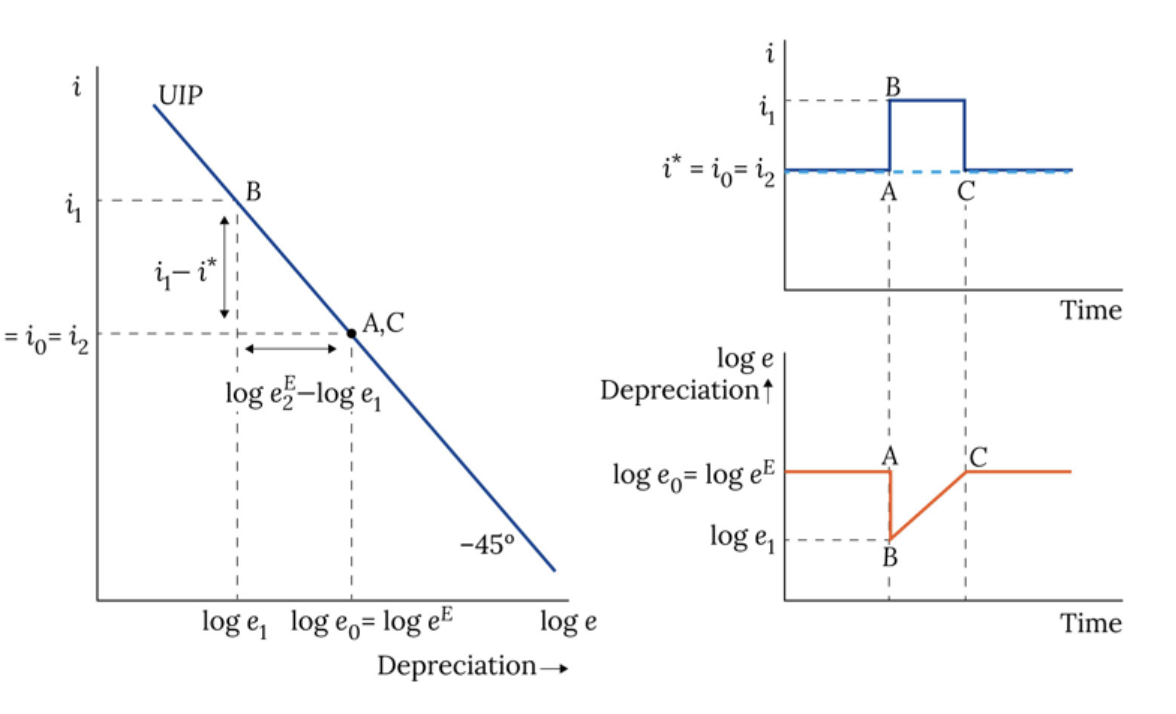
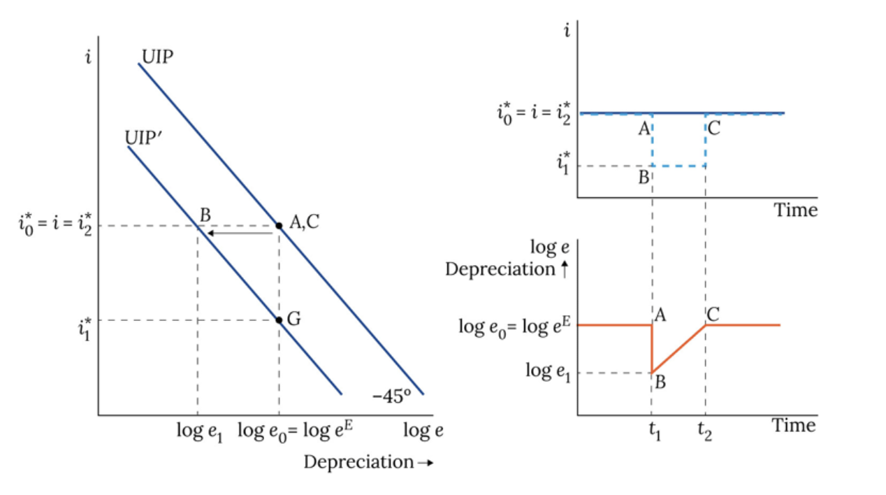
one period decrease in world rates with no change in exchange rate expectations

Start at A with home interest rate = world interest rate = i2 and exchange rate = expected exchange rate = e1. Now the world interest rate falls to i∗=i1 while the domestic interest rate remains at i2. There will be an immediate appreciation (a jump in the exchange rate) due to an increased demand for domestic bonds, reflecting the positive interest differential between home and world interest rates i2−i1=1. The exchange rate appreciates from e2 to e1. The UIP curve shifts and the economy moves to B.

The question states that the expected exchange rate remains unchanged at eEt+1, in which case the UIP condition is satisfied since the 45 degree line implies i2−i1=loge2−loge1. This UIP condition encapsulates the insight that, to ensure that purchase of domestic and sale of foreign bonds ceases, it must be the case that there is an expected depreciation that offsets the interest benefit of purchasing domestic bonds.

After the world interest rate reverts to its previous level at the end of period 1, the interest differential would revert to 0, UIP would shift back to its original position, and exchange rate expectations would be fulfilled by a return to point A.

CB loss functions

If the central bank cares only about inflation then the loss ellipses become one dimensional along the line at πt = πT.The value of β does not reflect whether the central bank focuses on achieving an inflation target or an output target. Rather, a central bank with lower β is willing to trade off a longer period during which inflation is away from target to reduce the impact on unemployment of the adjustment path back to equilibrium than would a more inflation-averse central bank with a higher β.

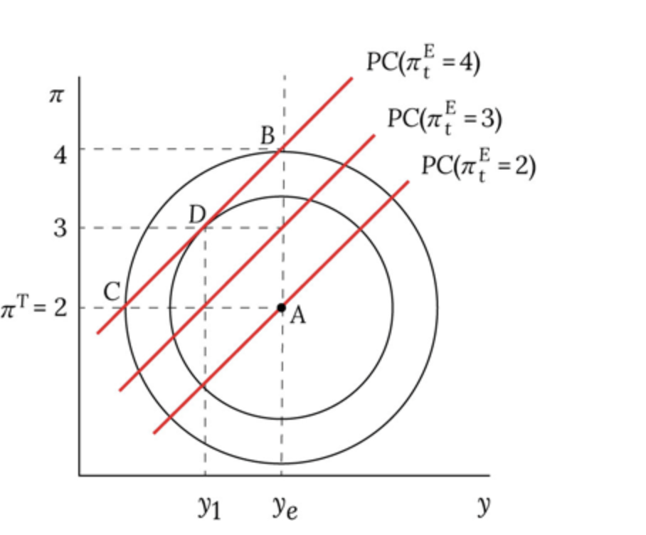
Loss curve and PC

In the diagram, it is assumed that α = 1, so that each Phillips curve has a slope of 45∘. If there’s an shock to inflation, bliss point is no longer obtainable, and CB faces tradeoff. Point B corresponds to a fully accommodating monetary policy in which the objective is purely to hit the output target (β = 0), and point C corresponds to a completely non-accommodating policy, in which the objective is purely to hit the inflation target.

given its preferences, if the central bank is faced by PC(πtE=4), then it minimizes its loss function by choosing point D, where the PC(πtE=4) line is tangential to the indifference curve of the loss function closest to the bliss point. Thus if its on PC(πtE=4) it will choose an output level y1 which will in turn imply an inflation rate of 3% and a Phillips curve the following period of PC(πtE=3)

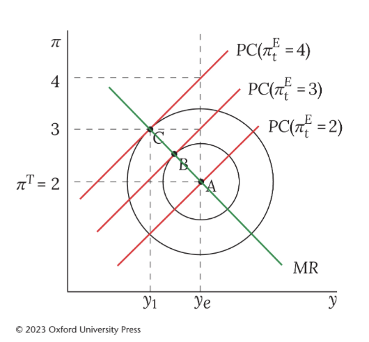
deriving MR from Loss function

1. Define the Central Bank (CB) preferences in terms of deviations from inflation target and equilibrium output. CB preferences are given by a loss function: L = (y_t − y_e)² + β(π_t − π^T)².
2. Define the CB constraints from the supply side i.e. the PC. The PC is a constraint for the central bank because it shows all the output and inflation combinations from which the CB can choose for a given level of expected inflation.
3. CB optimises at the best feasible tangency: slope of loss contour = slope of PC. Along any given PC constraint, choosing a point other than the tangency would lead to a greater loss.
4. Join these points to derive the MR curve.

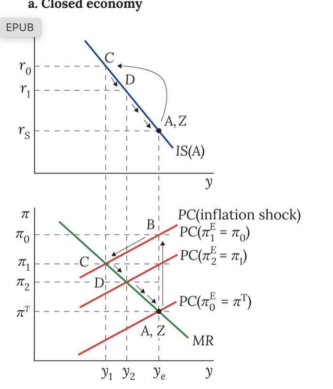
positive inflation shock (closed economy)

1. Inflation increases, shifting the PC upwards: A → B
2. CB chooses best-response output gap on MR at C and raises interest rate
3. Given the rise in unemployment, inflation falls, leading the PCto shift down
4. CB chooses best-response output gap at D and lowers the interest rate
5. CB guides the economy to Z by choosing its best response output gap along the MR and lowering the interest rate
6. At Z, economy is at equilibrium output and inflation is at target. The stabilizing interest rate is the same as at A. (note 1 period lag in output for IRF)

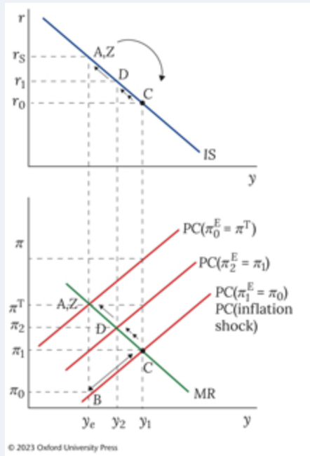
negative inflation shock

Period 0: We start at point A. A negative inflation shock shifts the Phillips curve to PC (inflation shock). Without an adjustment to the real interest rate, we end up at point B, which has lower inflation and the same output compared to A.

Period 1: The Phillips curve remains where it is. When the central bank can update the interest rate, they set it to get back on the MR curve and we end up at point C. This is movement along the IS curve from A to C by decreasing the interest rate. Output increases and inflation rises.

Period 2: The Phillips curve shifts to the left. The central bank will now move along the MR curve back towards the medium run equilibrium. In this period, we will end up at point D. Then this step will repeat until we return to the equilibrium.

negative permanent demand shock

negative permanent demand shock

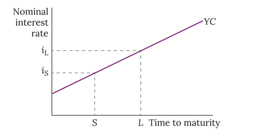
YC

An upward sloping yield curve indicates that yields on bonds of longer

maturity (e.g. 5 years) exceed yields on shorter-maturity bonds (e.g. 1

year). General implication: If markets are efficient, the return on a 5-year bond will be the

geometric average of the actual and expected returns on a series of 1-

year bonds bought and held consecutively over the next 5 years

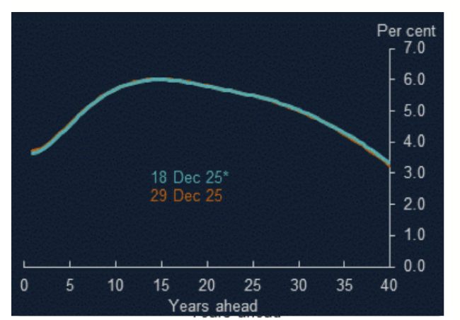
nominal yield curve BoE

The orange line (barely visible here) is the yield

curve on the date in question.

The turquoise line is the yield curve on the day of

the most recent MPC meeting, provided as a

reference point to see subsequent movements.

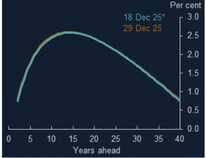
The instantaneous implied real forward curve (real interest rates):

The UK is one of a fairly small number of countries that issues index linked gilts. Those

are government bonds that guarantee that they will pay a nominal return and interest rate

coupon, but also compensate investors for inflation: the return that investors get rises

according to the CPI or RPI at the time. The fact that those bonds are protected from

inflation means that these bond prices will reflect expectations of real interest rates. So

the Bank of England is able to calculate a real terms yield curve, shown here.

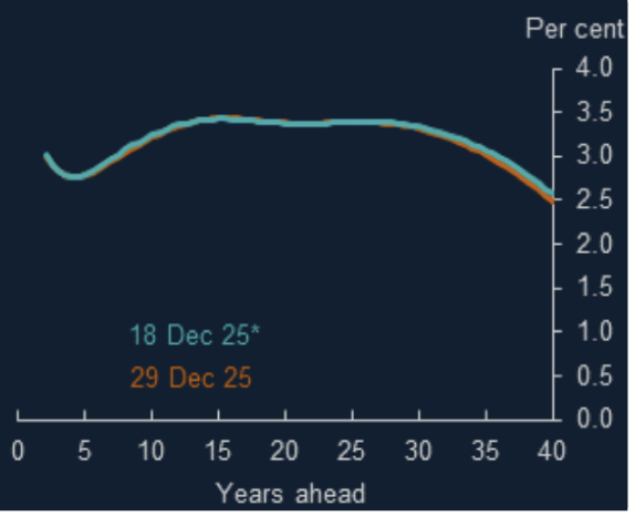
The instantaneous implied inflation forward curve (market inflation expectations):

The index-linked gilt market allows us to obtain real interest rates and the conventional gilt market allows

us to obtain nominal interest rates. These nominal rates embody the real interest rate plus a compensation

for the erosion of the purchasing power of this investment by inflation. The Bank uses this decomposition

(commonly known as the Fisher relationship) and the real and nominal yield curves to calculate the

implied inflation rate factored into nominal interest rates

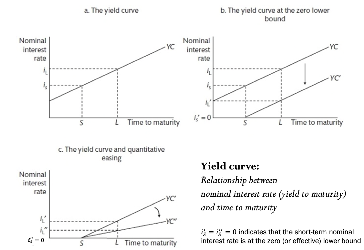
Policy interventions and the yield curve:

Panel a: Simplified yield curve (YC)

 2 types of bonds: short term (S) and long term (L), with interest rates 𝑆 and 𝐿.

 YC is drawn upward-sloping.

 In general, a positive slope will arise reflecting a higher risk premium from holding a bond over the longer

term due to uncertainty (‘term premium’). The slope of the curve is usually dominated by future interest rate expectations.

Panel b: Conventional monetary policy

 Central bank cuts interest rates in response to a negative AD shock.

 YC shifts down, but the spread between 𝑆 and 𝐿 stays the same.

 Even if 𝑆 (or slightly negative), 𝐿 might still be too high to stabilise the economy.

 The zero (or effective) lower bound has been reached.

 The level of 𝑖𝐿 is economically important because bank lending to the private sector is longer-term.

Panel c: Quantitative Easing

 YCʹ pivots down to YCʹʹ, and 𝐿 is reduced to 𝐿.

 QE can stimulate the economy to the extent that a lower 𝐿 boosts consumption and

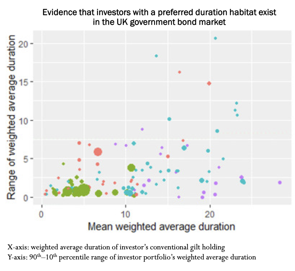
preferred habitat investors

Foreign central banks are present at the shorter end of the yield curve, largely

targeting duration habitats of 5 years or less

 Domestic banks are also concentrated at the shorter end of the yield curve

 Pension funds tend to target duration habitats of 15 years or greater

 Insurance companies sit somewhere between those two

These preferred habitat investors, who often hold the vast majority of

the stock of gilts, are less price sensitive than other investors.

 The tighter the habitat preference of the investor group, the less sensitive they are

to changes in the relative cost of a bond (increasingly inelastic demand).

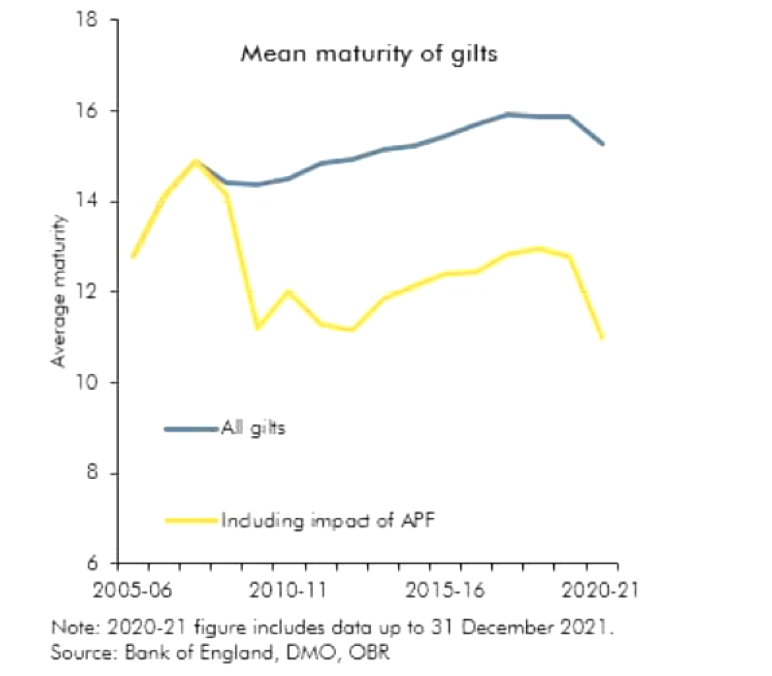
duration channel of QE. QE shortening maturity of available gilts

QE purchases of longer maturity gilts reduced the average maturity of

the remaining free float (yellow line). “All gilts” includes APF holdings.

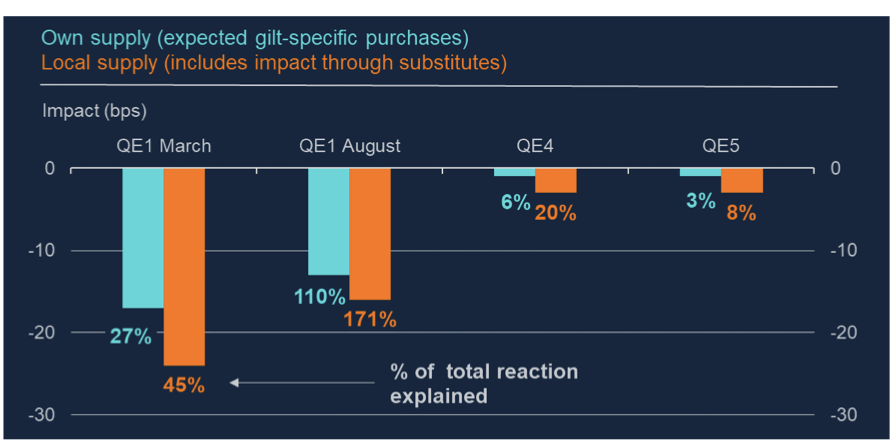
Portfolio rebalancing channel

When the central bank buys government bonds under QE, the available supply of those bonds in the market falls.
When supply falls, bond prices rise and yields fall.

The hypothesis:

• Bonds that the central bank is expected to buy should see bigger yield drops.

• Similar bonds (substitutes) should also experience yield declines.

Meaning:
A large portion of the yield fall came from broader market supply effects, not just the specific bond purchased. So QE works partly because it changes the supply of safe assets available to investors.

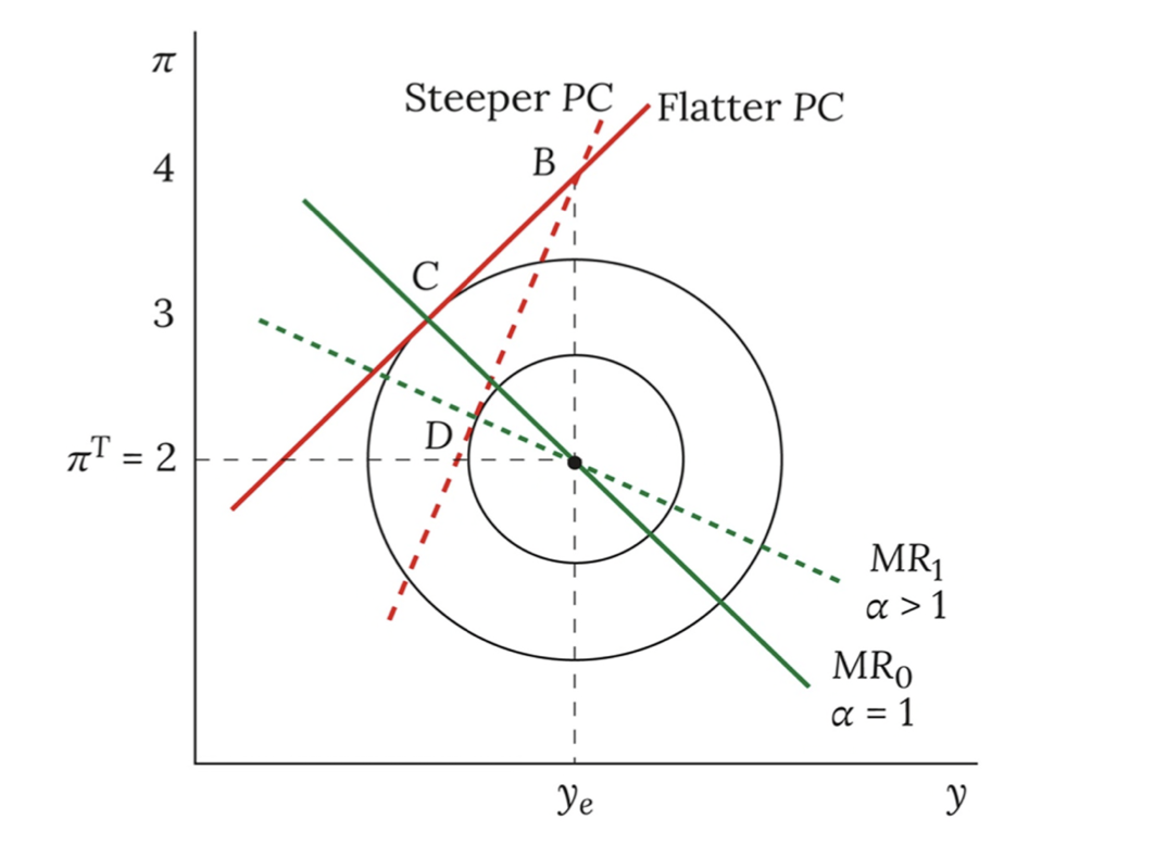
change in responsiveness of wages to unemployment PC

Responsiveness of wages to unemployment is represented by parameter 𝛼 in the wage setting equation. Intuitively, the policymaker facing a higher 𝛼 benefits from the higher responsiveness of wage setting

to (un)employment: nominal wage growth will respond rapidly to any change in unemployment (and

price inflation will match nominal wage inflation, and output and employment are assumed linearly

related). So the monetary policymaker requires a smaller output gap to achieve a given inflation

reduction. Note that the policymaker will exploit this, and – as the diagram illustrates – will choose a

larger inflation reduction (achieved with a smaller output gap) if the labour market exhibits this ‘more

flexible’ wage setting behaviour – the policymaker will be able to return the economy to the inflation

target and equilibrium output more quickly. Higher 𝛼 corresponds to a more flexible labour market

(which could reflect e.g. lower union power, lower efficiency wage considerations)

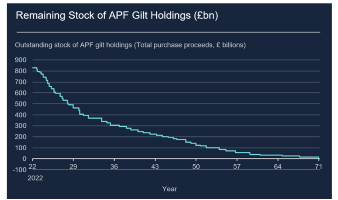
Passive QT

Even if not sold through active QT, APF gilt holdings would diminish as the gilts mature: eg The Bank of England (MPC)

stopped buying bonds at the end of 2021

stopped reinvesting the proceeds from maturing bonds in February

2022

announced in February 2022 that active bond sales would begin after

the September 2022 meeting

began actively selling bonds in the secondary market in November 2022

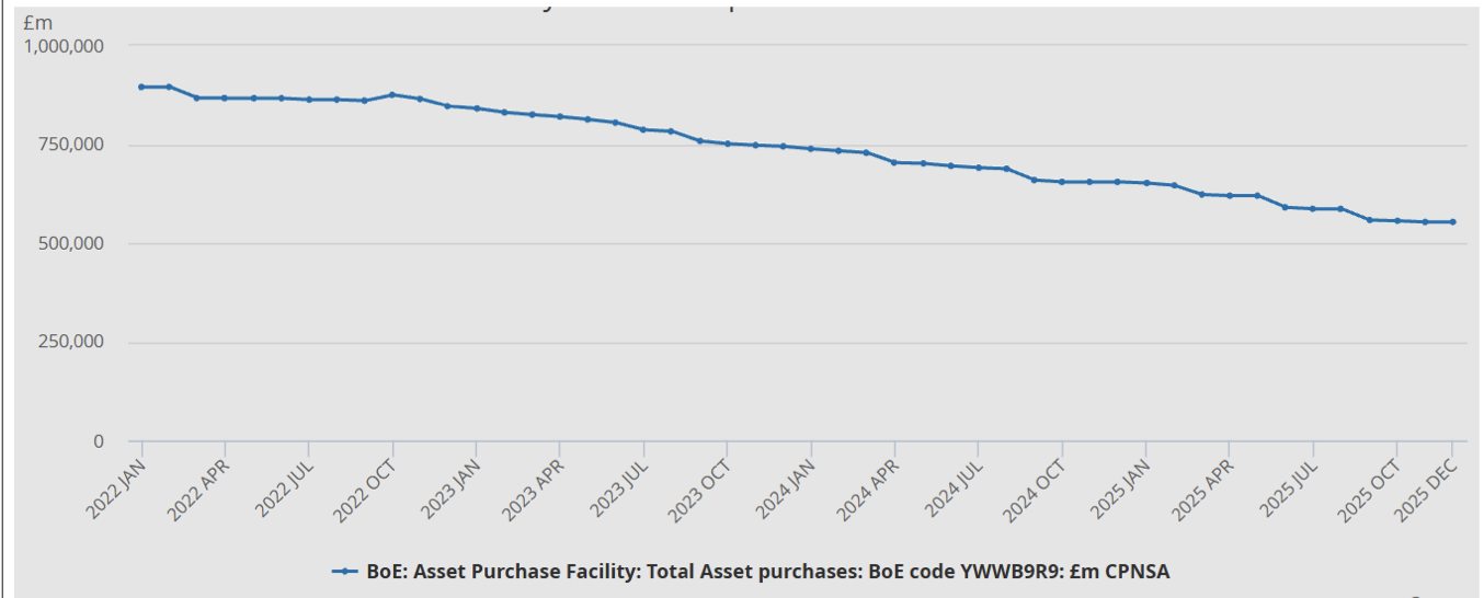
effect of QT on APF stock

Gilt sales gradually reduced the stock in APF from £894,939m in February 2022 to

£553,158m in December 2025.

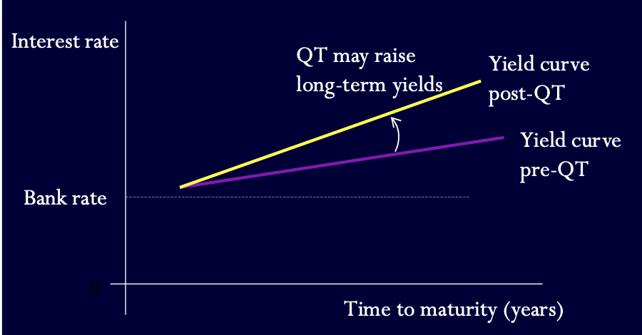
effect of QT on YC

The short end of the yield curve is pinned down by the policy rate.

 Any impact of QT will be at longer maturities. The yield curve might pivot

anticlockwise

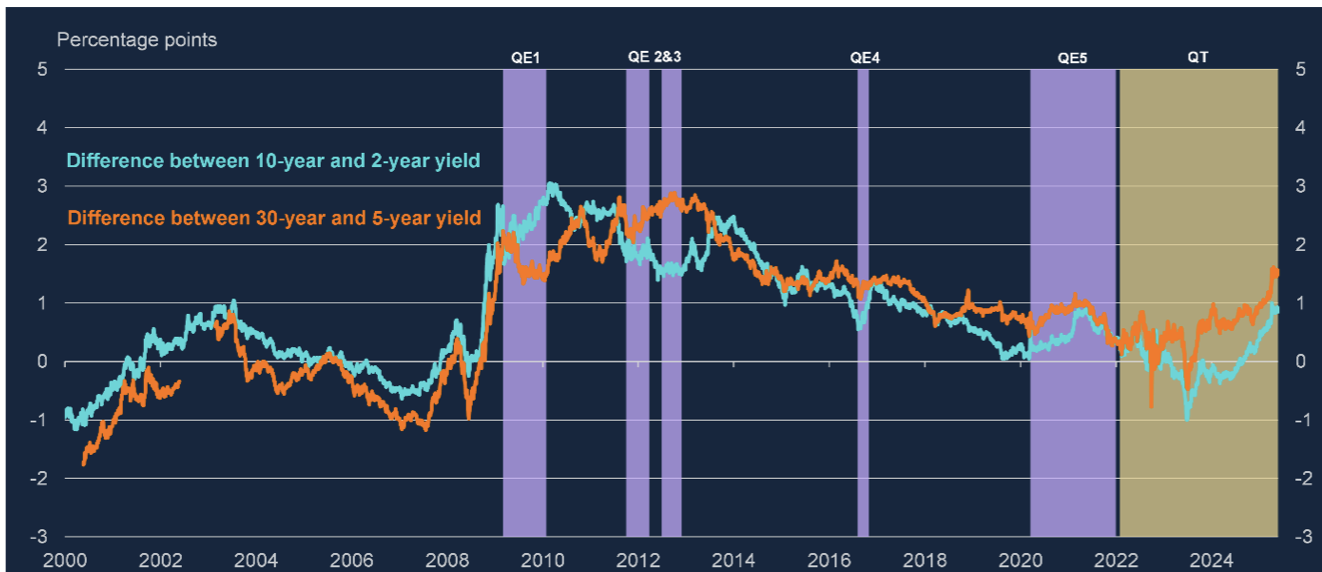
Effects of QT (and QE) on slope of yield curve

QT has been associated with a reversal of the decline in yield curve slope as

shown by differences between 2-year and 10-year and between 5-year and 30-year

conventional government bonds. Long-term bond yields have risen substantially

to leave the yield curve “unusually steep in historical context”

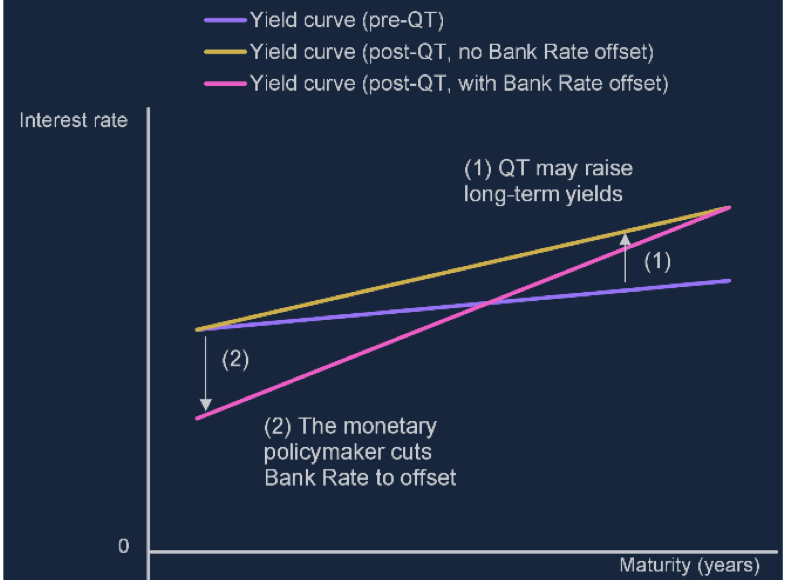
QT and conventional policy combined

Start at the purple line. The yellow line captures the impact of QT. The pink line is

the best effort possible via conventional policy to offset QT tightening.

 The purple and pink lines do not embody equivalent monetary stances, suggesting

it might not be possible to counteract QT by changes in the policy rate. This Mann (2025)

diagram shows conventional policy

only affecting the short end of the

yield curve. This may be valid,

since monetary policy operations

to implement Bank Rate affect

directly very short-term market

interest rates, so if these are not

transmitted via arbitrage to longer

rates, only the short end of the

yield curve will respond to

conventional policy changes.

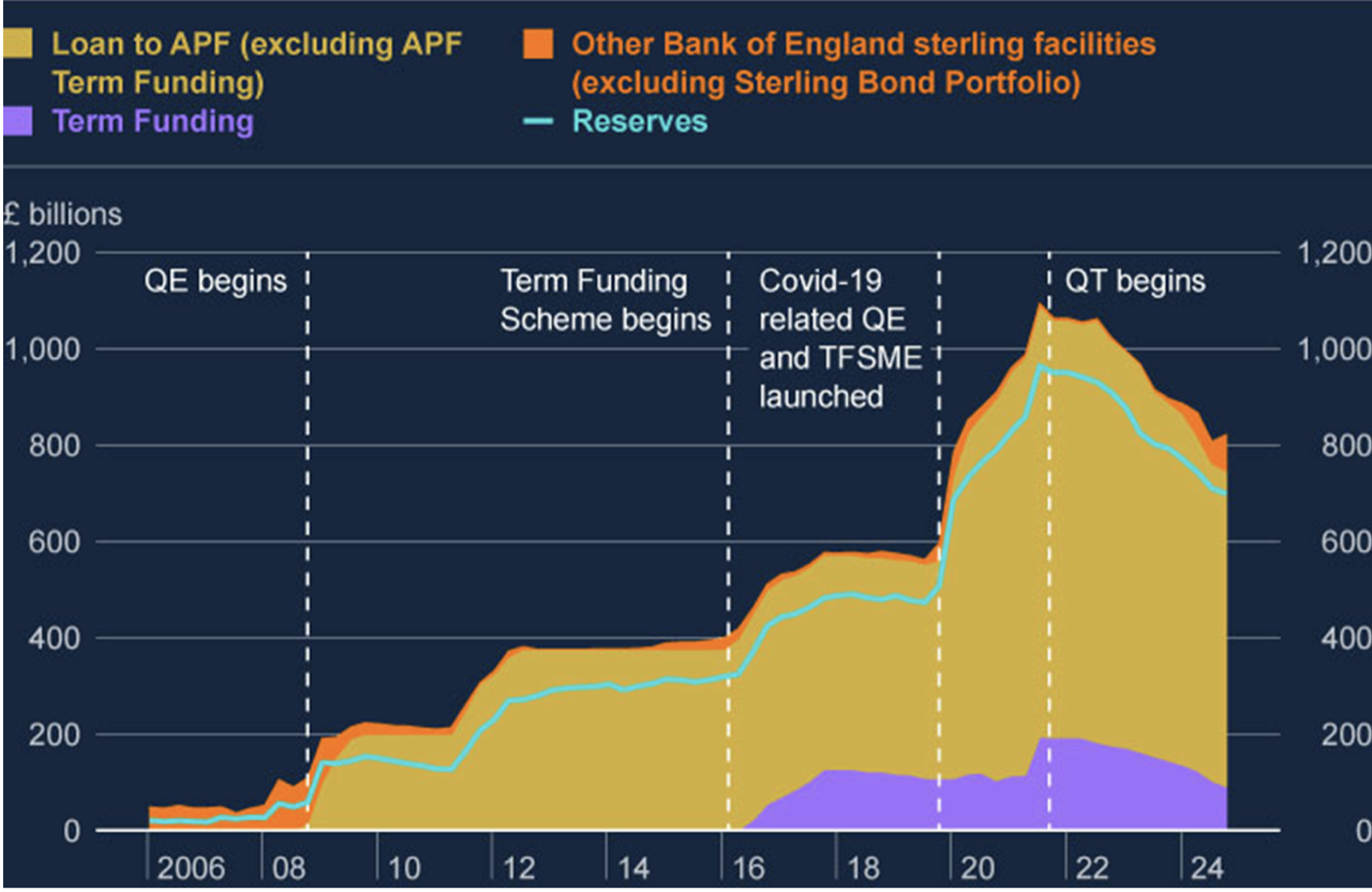
stock of reserves during QE and QT

during QT, stock of reserves falls.

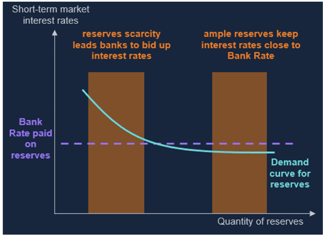
relation between demand for reserves and interest on reserves

Demand for reserves is negatively related to the difference between

other interest rates (on other liquid assets) and interest on reserves. The diagram shows how a central bank (e.g., the Fed, Bank of England, ECB) can keep short-term market rates near its policy rate by supplying ample reserves. Scarcity would cause volatility and higher rates, while ample reserves create a stable, rate-controlled environment.

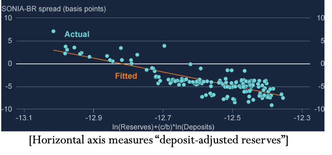
relation of SONIA-BR and demand for reserves

as market rates, SONIA𝑡, rise relative to

Bank Rate, BR𝑡, the demand for reserves falls, for any given level of deposits. The BoE estimates suggest that a 10% decrease in aggregate reserves is

associated with a 1.5 basis points increase in SONIA relative to BR, all

else equal. (OLS estimate)

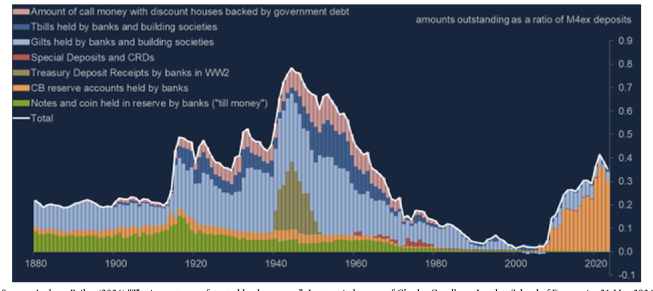
Commercial banks’ safety buffers: liquid assets held

by banks and building societies 1880-2024

The chart shows that assets considered as “safe” (i.e. liquid, reliably backed) held

by banks and building societies, as a ratio of deposits, fell to low levels pre-

financial crisis.  Safe assets include reserves, government-backed assets including gilts and T-bills, notes and coin.

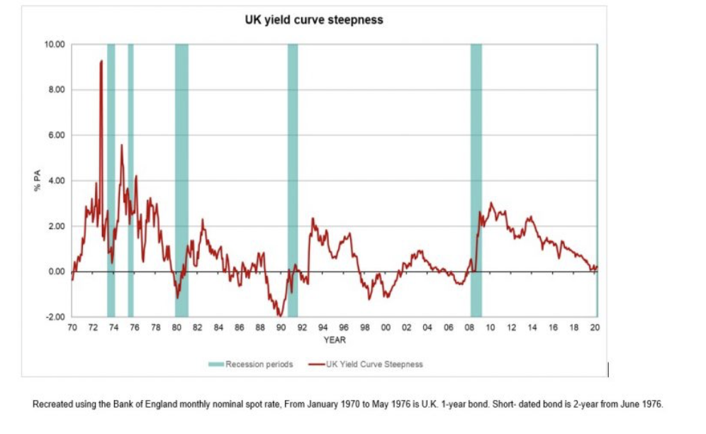
downward sloping YC

At the short end of the maturity spectrum, the imminent recession might be accompanied by an increase in perceived gilt risk (e.g. price volatility, currency risk for foreign holders, default risk - though default risk is effectively zero for countries like the UK). This would raise short-term yields. At the long end of the yield curve, government bond prices might reflect increased demand due to a “flight to quality”: before a recession, riskiness of other long-term assets (corporate bonds, property) might be perceived to rise, so investors rebalance their portfolios to include more, safer, gilts. The increase in demand for long term bonds results in a fall in the yields at the long end of the yield curve.

Also, the formula from above  (1+𝑖5𝑡)5=(1+𝑖1𝑡)(1+𝑖𝐸1𝑡+1)(1+𝑖𝐸1𝑡+2)(1+𝑖𝐸1𝑡+3)(1+𝑖𝐸1𝑡+4) indicates that inversion may be associated with a belief that policy now is considered tighter than it is expected to be in the future: 𝑖1𝑡>𝑖𝐸𝑡+𝑛. (expected future rate cuts) This could be because financial markets judge that a recession is coming and policy will have loosen, or that policy is too tight now and will induce a recession.

home rate above world rate for 1 period (w UIP)

Assuming expected exchange rates are fixed, due to the home interest rate being above world rate, actual exchange rate must change. According to the UIP condition, as soon as the interest rate differential opens up, home’s exchange rate will appreciate immediately (jump) to loge1 so that its expected depreciation over the year is equal to the interest rate differential. In the left-hand panel of Figure 11.3, the two double-headed arrows are equal in length. The impulse response function highlights the fact that the interest rate differential persists for one period and that the exchange rate jumps as soon as the news of the interest rate differential arises. During that period, the nominal exchange rate depreciates.

fall in world interest rate shifts UIP (foreign recession)

A foreign recession:
1. Initial equilibrium at point A.
2. UIP curve shifts left because there has been a fall in world interest rate.
3. A → B: home’s interest rate now above world interest rate, arbitrage in financial markets will lead to an immediate appreciation of the home exchange rate
4. B → C: Over the course of the year during which there is an interest gain on home bonds, home’s exchange rate depreciates
5. C: At the end of the period, world interest rate reverts to initial rate and UIP curve shifts back. There is no interest differential and exchange rate is at initial rate.

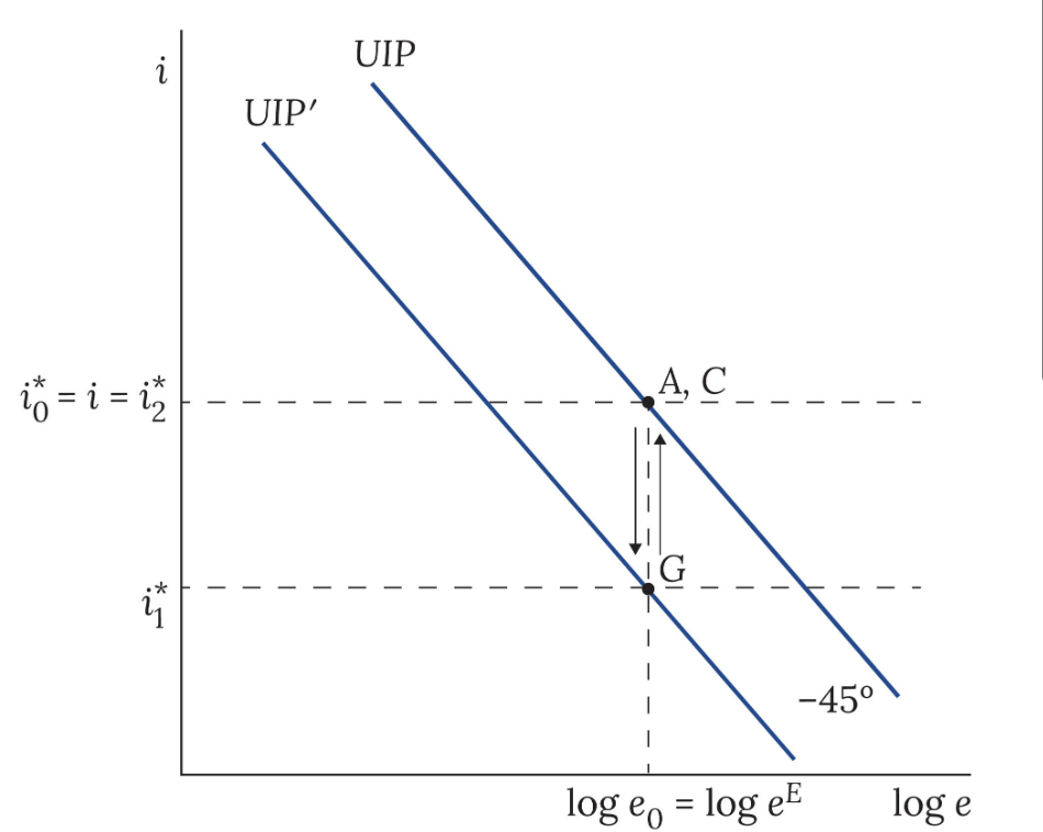
global recession, CB matches world rate

1. Initial equilibrium at point A
2. UIP curve shifts left because there has been a fall in world interest rate
3. A → G: home CB immediately matches foreign CB so that i = i₁^*. No exchange rate change
4. At the end of the period, world interest rate reverts to initial rate and UIP curve shifts back. Home again matches foreign CB, then G → C and the exchange rate doesn’t change. so on IRFS (log e is unchanged throughout)

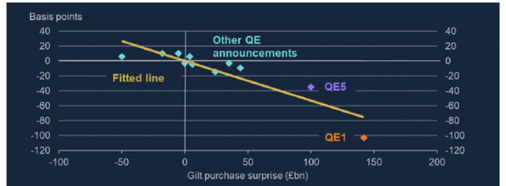
Change in 10-year gilt yields after QE announcement and gilt purchase surprise

Anticipated QE purchases would already be factored into (reflected in) gilt yields so yields will only move

(further) in response to unexpected purchases. Even under these assumptions, QE could have an impact if

it signalled future interest rate policy, leading to a change in expected future interest rates, which are a

component of long bond yields. For QE to work, yields should fall. The purple and orange points indicate that QE1 and QE5 had both

large elements of surprise (far to the right on the horizontal axis) and large yield changes (vertical axis

shows about -40 and -100 basis point change in yields respectively). The other QE announcements show

much less surprise and lower changes in yields.

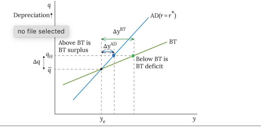
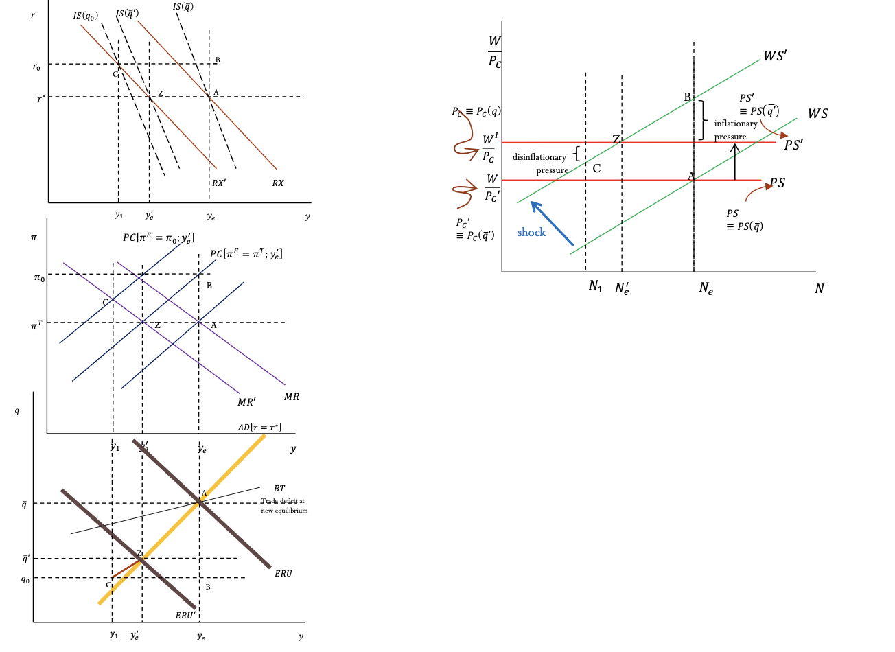
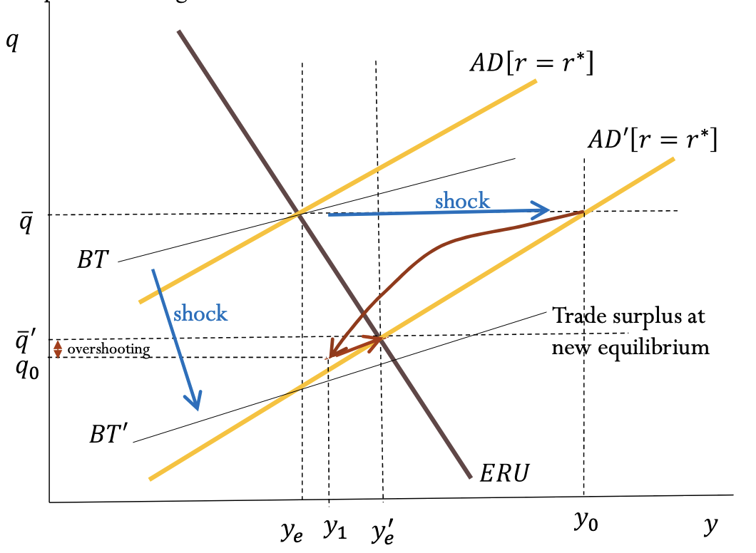
deprivation in BT/AD

Net exports rise. Equilibrium

output rises by 𝐴𝐷. At the new equilibrium, there is a trade surplus (AD is above BT).

 The trade surplus arises because the boost to output (multiplier effect of net export rise) is not

sufficient to suck in imports equivalent to the depreciation-induced higher exports, since only a proportion

(marginal propensity to import ) of the higher output is spent on imports.

 The new goods market equilibrium is at a lower income level than the new balanced-trade level of output .

A much larger income rise would be required to suck in an amount of imports equivalent to the higher net exports that have resulted from the depreciation, to get to trade balance.

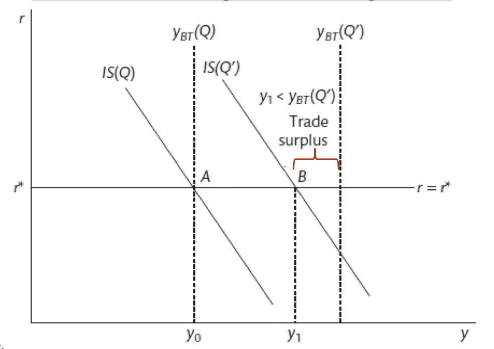
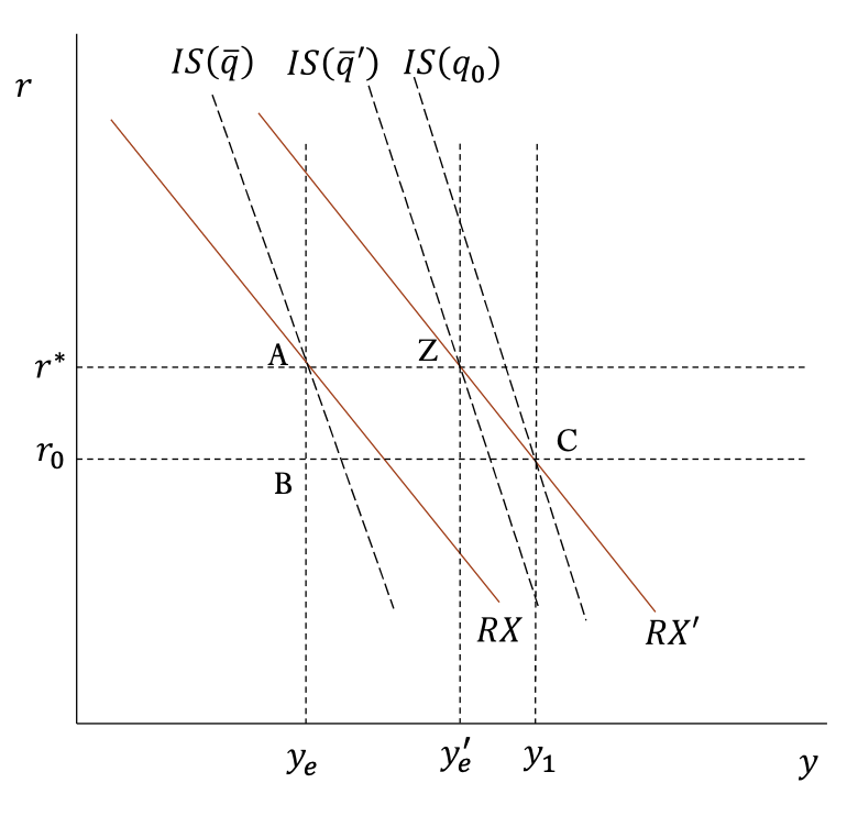
impact of a real depreciation on equilibrium output and the balanced trade level of output yBT and existence of a trade surplus at the new equilibrium

The real exchange rate

depreciation shifts the

IS curve right in

r-y space: this is how

the rise in equilibrium

income resulting from

the consequent rise in

net exports is

graphically

represented.

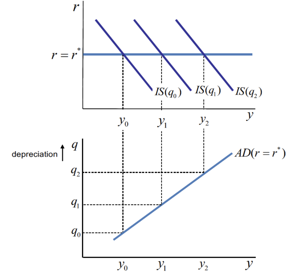
Derive the AD curve graphically from the IS curve.

We know that 𝑟 must be equal to 𝑟∗ on a given AD curve, so to derive the AD curve from the IS curve we need to vary 𝑞and see what happens to the intersection of the 𝑟=𝑟∗ line and the IS curve. The top panel of the graph below shows how the IS curve shifts to the right with a more depreciated exchange rate, where 𝑞2>𝑞1>𝑞0 . If we trace these combinations of 𝑞 and 𝑦 onto the bottom panel of the graph below, we can derive the AD curve.

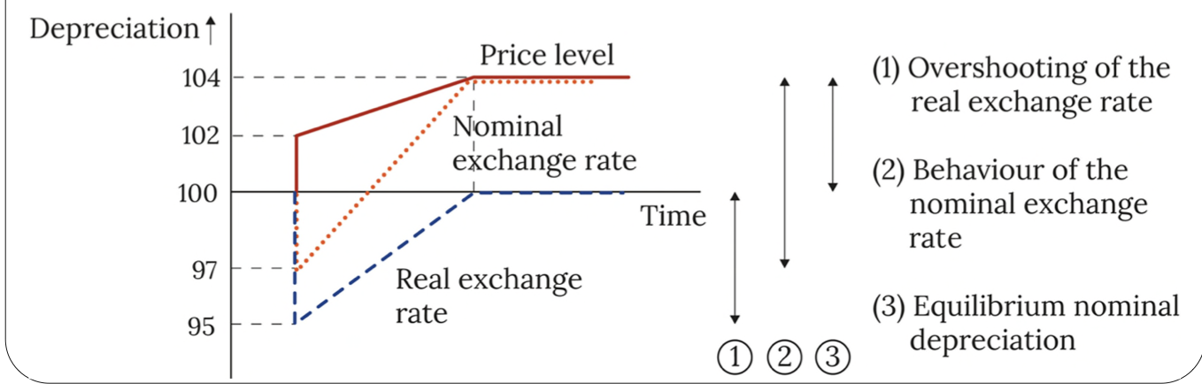
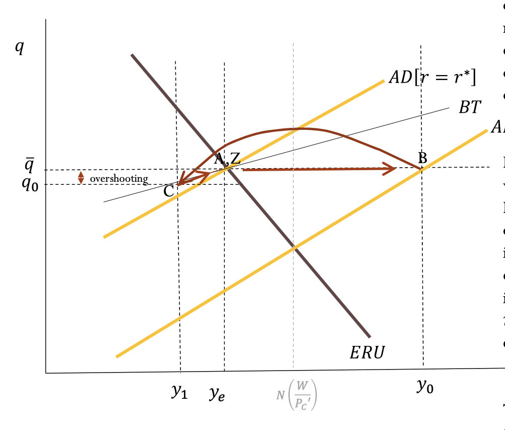
exchange rate overshooting

An inflation shock does not alter the equilibrium real exchange rate.

 Prior to the shock, P, e and Q, are constant at 100. The constancy of P is consistent with the domestic policymaker targeting 0% inflation.

 The values of e and Q imply that the world inflation rate is also initially 0%, and we assume it remains 0% throughout.

The inflation shock raises prices from 100 to 102, a 2% increase.

The inflation targeting home policymaker raises the real interest rate above the world level until

inflation is back at its 0% target.

r>r∗ leads to an immediate real exchange rate appreciation, falling from 100 to 95.

An inflation shock does not alter the equilibrium exchange rate, so following its initial jump the

real exchange rate gradually depreciates while r>r ∗, eventually returning to the original equilibrium value of 100

summary

The initial nominal appreciation < initial real appreciation since the inflation shock (price level rise) contributed some of the required real exchange rate appreciation.

• Real depreciation reflects r>r∗ (real UIP condition).

• During adjustment, nominal depreciation > real depreciation. Reflecting the formula for Q, the

nominal depreciation has to be larger than the real depreciation to offset the real appreciation that happens because P continues to rise (inflation>0) as inflation falls back to target.

The nominal exchange rate e can be regarded as a ‘residual’ as it simply moves according to the definition:Q = 𝑃∗𝑒/𝑃.

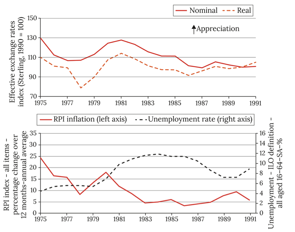
Exchange rate overshooting during Thatcher recession

Exchange rate overshooting during the Thatcher recession 1980-82: Tightening

of monetary policy (MTFS, 1979) did not lead to an immediate fall in inflation, but instead

led to a sharp appreciation of the pound £, because the forex market anticipated a prolonged period ofhigh real interest rates.

The exchange rate jump (overshooting) worsened UK competitiveness,

reduced exports and is viewed as havingcaused permanent damage to manufacturing sector, leading to a substantial rise in unemployment.

positive inflation shock with policy response (vertical ERU)

1. Initial equilibrium at point A
2. Inflation increases, shifting the PC upwards: A → B.
3. CB chooses best-response output gap on MR at C. To implement its policy, it raises the interest rate to C on the RXcurve as both forex agents and CB know the interest rate rise will be accompanied by an appreciation (and leftward shift of the IS) that will shoulder some of the burden of adjustment.

( The real exchange rate jumps immediately and will depreciate while the home interest rate is above the world level. During adjustment, the economy follows a path back to equilibrium consistent with AD(𝑟 = 𝑟𝑡) where 𝑟𝑡 ≠ 𝑟∗)
4. CB chooses best-response output gap at D and lowers the interest rate; IS shifts right as real exchange rate depreciates
5. CB guides the economy to Z along MR and RX
6. At Z, economy is at equilibrium output and inflation is at target. The real exchange rate is the same as at A.

7. Note that there is a second AD line that goes through points A, C, D. This is the AD(r = r_t) line, showing the level of AD associated with a given q when r = r_t. It is shown in dashed grey.

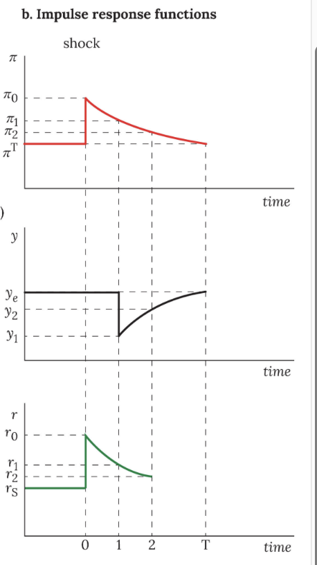
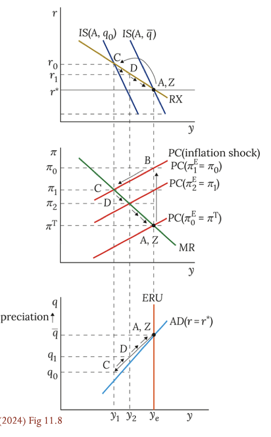
open economy positive inflation IRFs

period 0 interest rate can only affect economic output with a one period lag, however, so the economy ends period 0 with inflation at π0, output at ye and interest rates at r0.

period 1: the economy ends period 1 with inflation at π1, output at y1 and interest rates at r1.

period 2 onwards: The adjustment to the inflation shock ends when the economy is back at point Z, with output at ye, inflation at πT and the interest rate at rS.

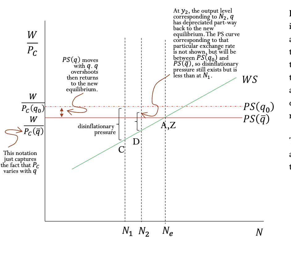
inflation shock with policy response W/Pc curve

If policy responds by raising

interest rates above world level,

as shown in the panel,

the PS curve will shift up

temporarily, following the

temporary exchange rate

appreciation, then return to its

original level as the exchange

rate depreciates.

There is disinflationary pressure

at N1 and N2, which correspond to y1 and y2

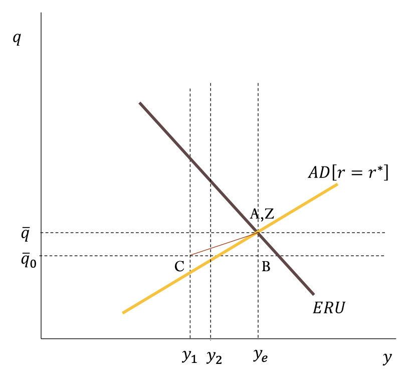
inflation shock with policy responses AD/ERU curves

The FOREX market and so the real

exchange rate respond immediately to

the shock and expected policy

response. The changes in q and r have

lagged impacts on net exports and

interest-sensitive spending,

respectively, so y changes with a lag.

The BT curve is not shown. BT does not

shift. Trade is balanced before and after

the shock.

intercept of BT equation(value of yBT when q=0,) shows that

BT only shifts with changes in α or Y*.

If monetary policy responds by raising

the interest rate, as shown in the r-y

panel, the economy will be off the AD

curve while r>r∗

.

Negative supply shock via WS – with policy response

The central bank responds to the

inflationary pressure induced by

the shock by raising the real

interest rate to the level consistent

with its chosen negative output

gap.

The IS curve shifts with changes in

the real exchange rate (noting that

net exports respond with a lag to

changes in q).

The real UIP condition holds at all

times. After the shock, the

expected equilibrium real

exchange rate is(qbarprime). As an example

of the real UIP conditions that hold

as q and r return to their

equilibrium levels, at the time of

the shock, period 0, the real UIP

condition is qbarprime-q0 =ro-r*

MR/PC: There is inflationary pressure at B

as the wage setting curve has

shifted up/left, so at the current

employment level, workers

demand higher nominal wages.

This is captured here as the PC

where inflation expectations are on

target will now intersect the new

equilibrium output, so is above

pi𝑇 at the old higher equilibrium

output.

The CB’s bliss point is at intersection of

pi𝑇 and y𝑒 so MR shifts with y𝑒.

The central bank forecasts the

inflationary pressure and chooses

negative output gap y1-y𝑒’, creating disinflationary pressure.

Inflation expectations and the PC

will gradually fall, allowing the

central bank to reduce the output

gap until the new equilibrium is

reached.

WS: The shock shifts WS up/left. At the current employment level, workers demand higher nominal wages,

generating inflationary pressure. The central bank responds; the negative output gap corresponds to

employment level N1, below new equilibrium employment N𝑒’, which generates disinflationary pressure. The shock and policy response lead to an immediate shift in PS, as the exchange rate jumps.

The post-overshooting PS movement to final equilibrium happens gradually as the real exchange rate depreciates from its overshooting level back to its new

Only initial and final PS curves are pictured here.

AD/BT: The negative supply shocks leads to lower equilibrium

output and an appreciated equilibrium exchange rate. During the period of policy action, r>r∗. The exchange rate overshoots. The economy

is off the AD curve. For given q, output is below where it would be if r=r∗. For given output, q is less appreciated

than it would be if r=r∗

(the higher net exports

balancing the lower

investment, compared to a

situation where the economy

was on the AD curve).

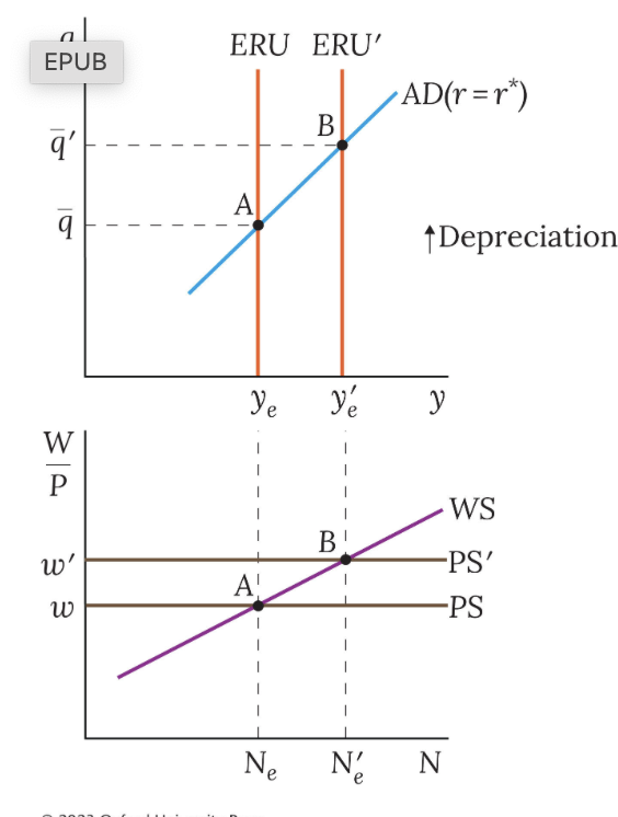
+ve supply shock on medium run exchange rate
(vertical ERU)

1. Initial equilibrium at point A
2. Improvement in productivity shifts the PS up and hence, ERU shifts to the right
3. New equilibrium is at B at higher output, a depreciated real exchange rate and a higher real wage
4. For output demanded (on AD ) at B to be equal to the new higher level of supply at y'_e, then given r = r*, the higher demand must come from a depreciated real exchange rate raising net exports.

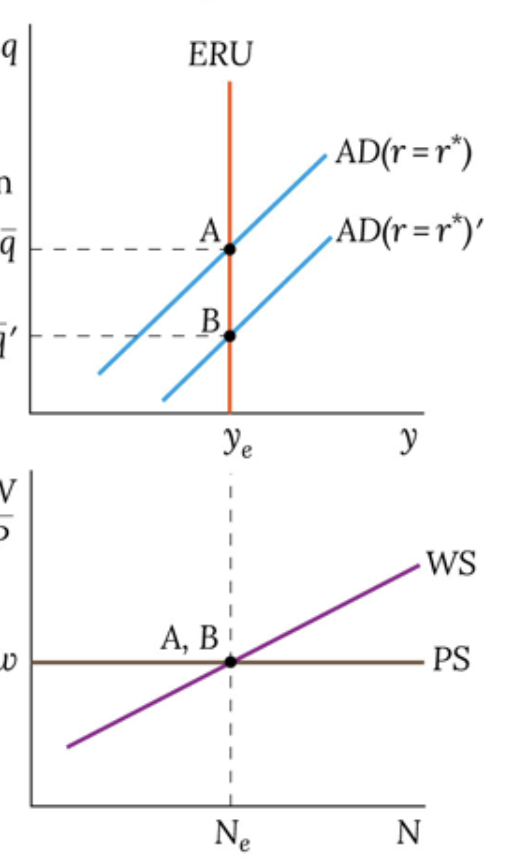
positive demand shock on medium run exchange rate
(vertical ERU)

1. Initial equilibrium at point A
2. Investment boom shifts AD curve to the right
3. New equilibrium is at B with an appreciated real exchange rate. Output is unchanged as no change on supply side
4. Since output is unchanged, the positive effect of the investment boom on output demanded must be offset by lower net exports, achieved by an appreciated exchange rate.

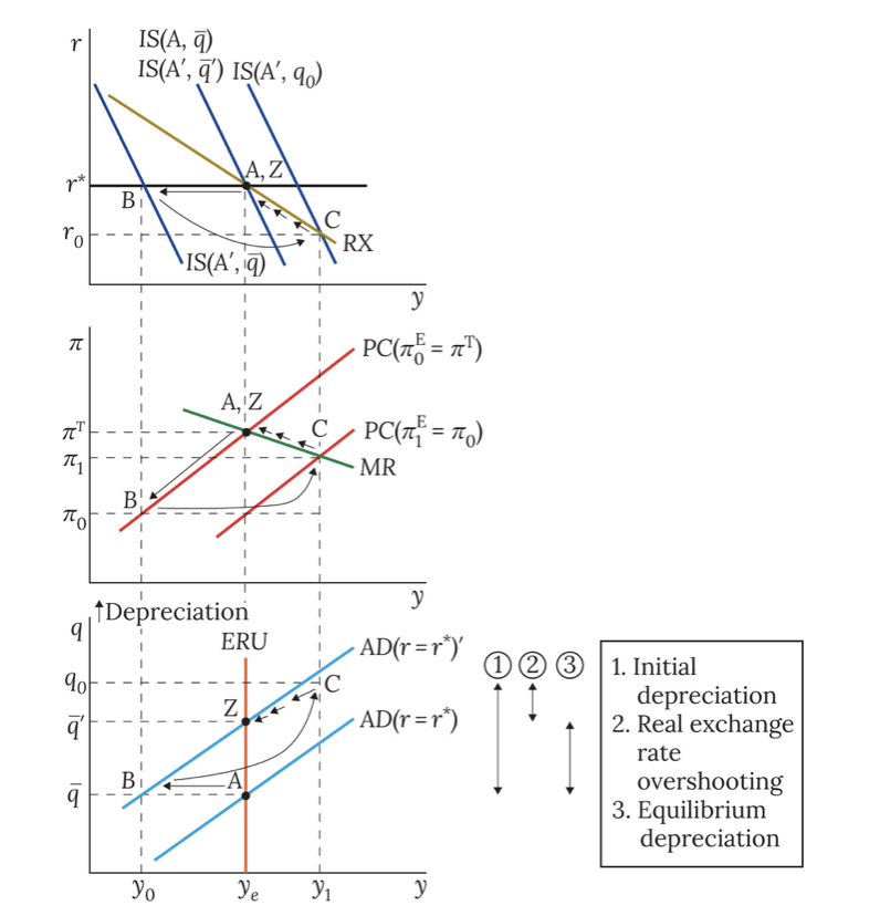
dynamic adjustment to negative perm demand shock
(Vert ERU)

1. Initial equilibrium at point A
2. IS shifts left, output and inflation decrease; A → B
3. CB chooses best-response output gap on MR at C on MR. Forex market anticipates CB will keep interest rates below world interest rates to boost demand, causing immediate depreciation of home currency. ISshifts right as CB sets r on RX at C.
4. At C, IS has shifted further to the right than the original IS (and new equilibrium) curve. The initial depreciation includes real exchange rate overshooting.
5. C → Z adjustment follows process detailed in Fig 9.8b. IS curve gradually shifts to the left and economy moves along the MR and RXcurves as CB adjusts the interest rate upwards back to r^* and exchange rate appreciates.
6. At new MRE, the real exchange rate is depreciated by the amount required to replace the permanently lower private demand.

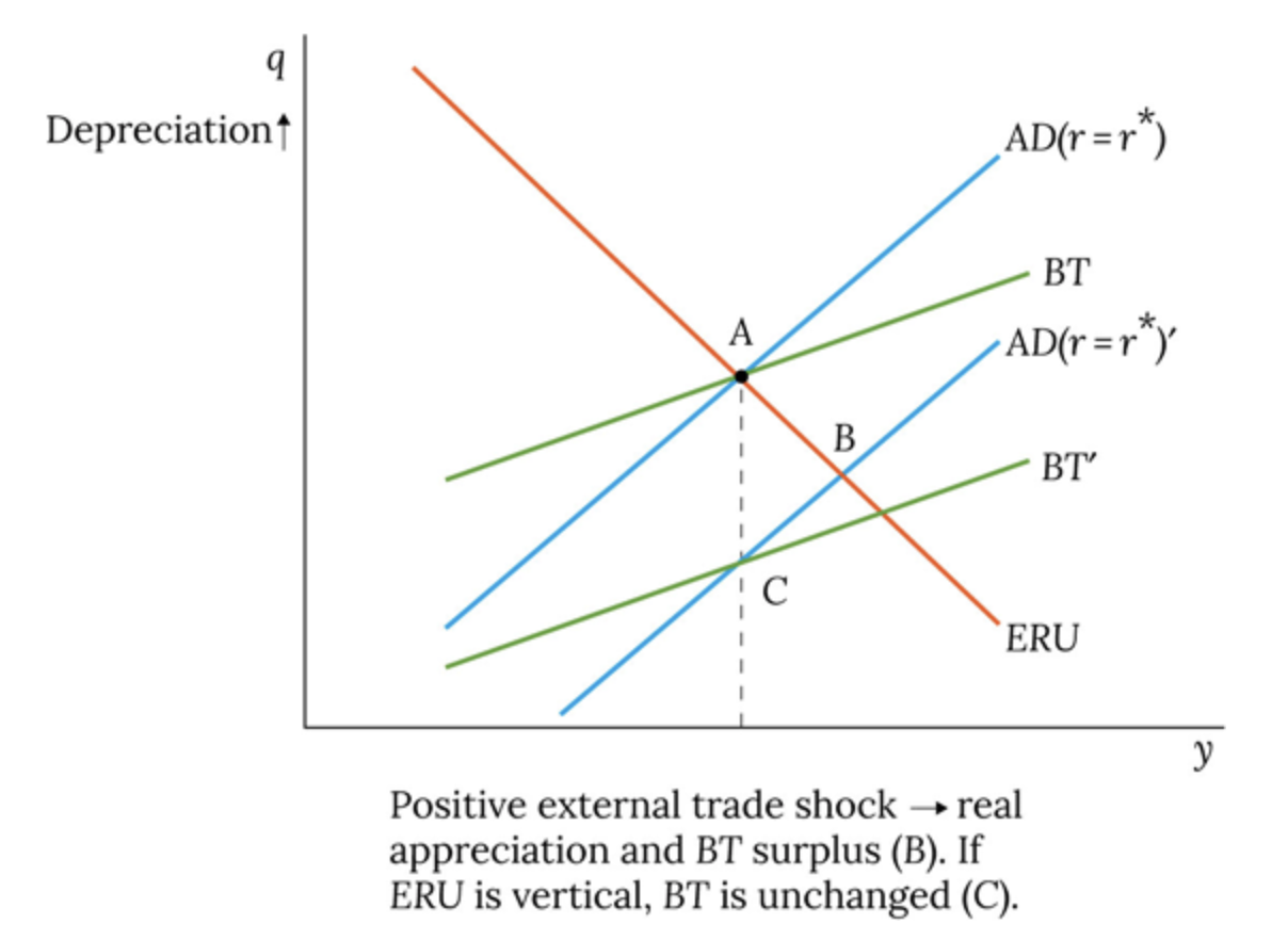
positive external trade shock

1. Initial equilibrium at point A.
2. The positive external trade shock raises net exports (rise in σ or y^*), which shifts the AD curve shifts to the right and the BT curve to the right.
3. Under a vertical ERU, new equilibrium is at C which is where AD' and BT' intersect. At point C, the appreciation of the RER is such that it causes net exports to fall by the exact amount that the external trade shock increases them. Trade is therefore balanced at point C and output is unchanged.

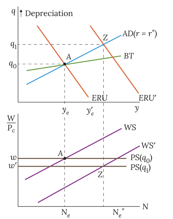
positive supply shock via WS

1. We start at equilibrium point A.
2. Step 1. Locate the new ERU curve. As before, the positive supply shock shifts the WS curve downwards. Point B at the WS-PS intersection for PS(q₀) will be on the new ERU.
3. The rightward shifted ERU curve goes through point B (see previous slide)
4. Step 2. Locate the new AD — ERU. intersection at Z. To achieve this output with a downward-sloping ERU, the exchange rate would have to depreciate to q₁. This shifts PS(q) downward (higher real cost of imports reduces the real wage).
5. Unlike the case with the vertical ERU curve, the real wage in the new equilibrium at Z is lower than at A.
6. At Z, the economy is above the BT curve, so there is a trade surplus.

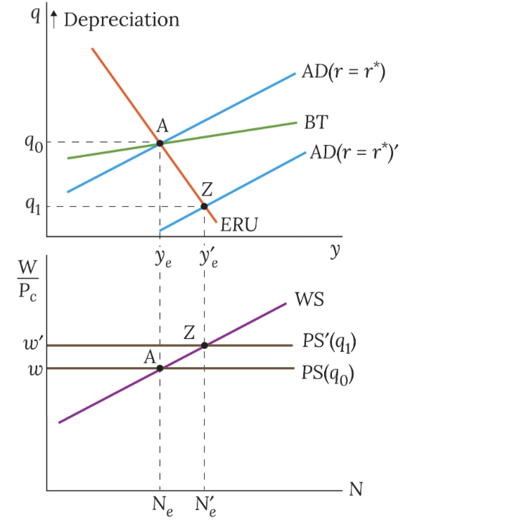
positive demand shock diaganol eru

1. We start at equilibrium point A.
2. A positive demand shock, shifts the AD curve to the right.
3. The new equilibrium at Z is at higher output: this implies a higher real wage is necessary (as shown by the WS curve). This requires a lower cost of imports, i.e. an appreciated RER.
4. At Z, there is higher domestic demand but lower net exports. There is a deficit on the balance of trade for two reasons — higher imports because of higher output and lower net exports because of lower competitiveness.

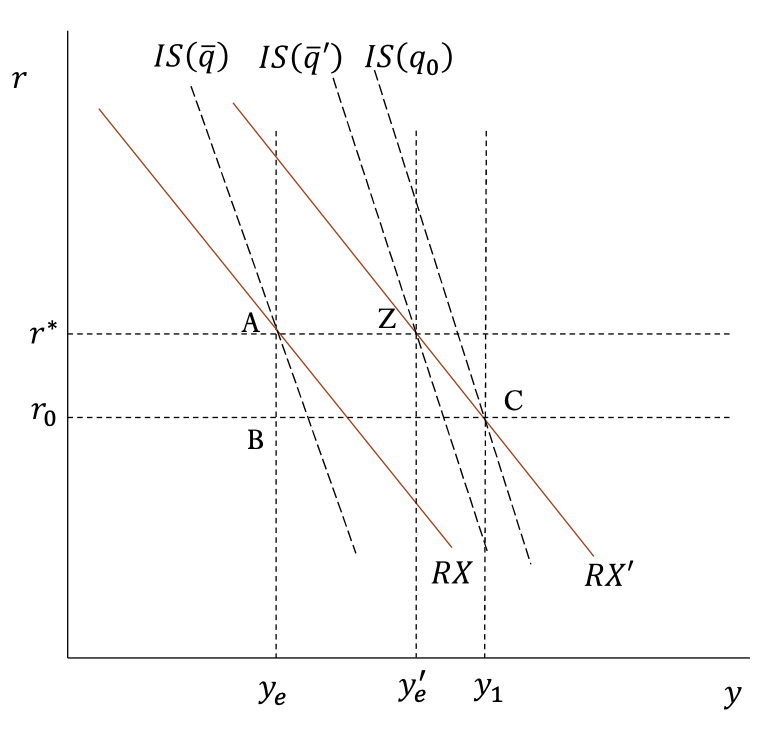
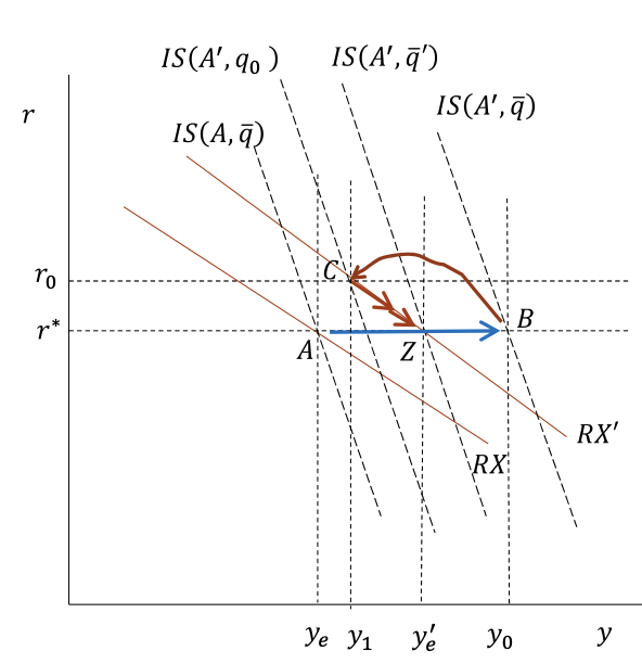
+ve supply shock policy response (via PS) (IS/RX)

The central bank responds immediately to the

disinflationary pressure induced by the shock by

reducing the real interest rate to the level

consistent with its chosen positive output gap.

There is no immediate change in

demand/output following the policy reaction to

the shock, because interest-sensitive spending

responds to changes in 𝑟 with a lag.

The real exchange rate responds immediately to

the shock and policy response. Exchange-rate

sensitive spending has a lagged response to

changes in 𝑞.

The real UIP condition holds at all times. After

the shock, the expected equilibrium real

exchange rate is ̅𝑞′. As an example of the real

UIP conditions that hold as 𝑞 and 𝑟 return to

their equilibrium levels, at the time of the shock,

period 0, the real UIP condition is ̅𝑞′− 𝑞0 = r0-r*

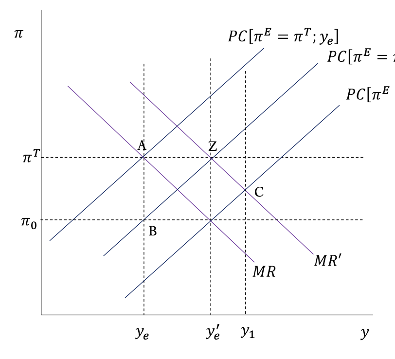
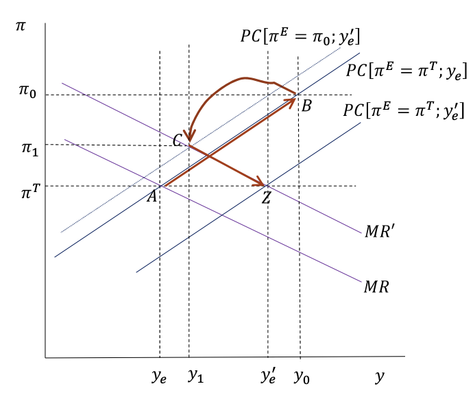
+ve supply shock policy response (via PS) (MR/PC)

Output does not change

immediately following a supply

shock because supply shocks

work via the labour market and

labour supply decisions are based

on previous period data so there

is no immediate change in

employment and output.

The central bank forecasts the

new MR curve and next period’s

Phillips curve, which will

correspond to new equilibrium

output and the period-0 inflation

rate . The CB chooses a positive output gap consistent corresponding to MR’, and the adaptive expectations PC that reflects inflation expectations after shock (pi0,ye’) and sets r0. In subsequent periods, inflation

expectations adjust, the central

bank modifies the interest rate

accordingly, and the economy

returns gradually to the inflation

target at the new equilibrium

level of output.

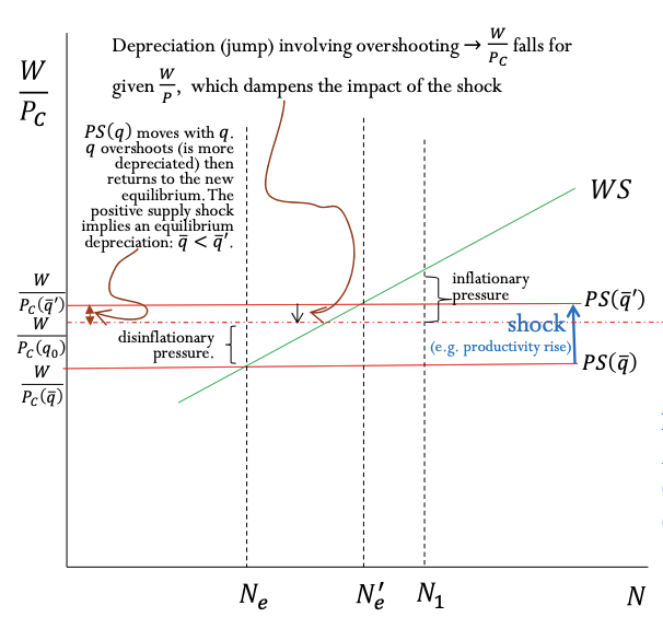
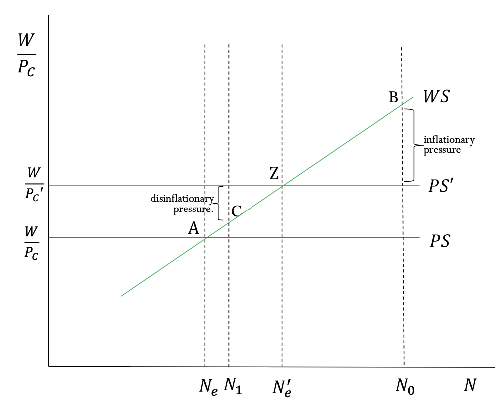
positive supply shock via PS (ws curve)

The shock shifts PS up. At the current employment level N𝑒, too few workers are offering their labour,

given the higher real wage. Nominal wage demands are too low, relative to the wage consistent with

pricing decisions. WS<PS corresponds to disinflationary pressure. The central bank responds with a real

interest rate reduction and positive output gap, employment rises to N1, where there

is inflationary pressure.

Exchange rate movements (the exchange

rate channel) reinforce the impact of

interest rate changes.

Inflation gradually returns to target, and

output and employment gradually fall

back to their new equilibrium levels. (can omit q0 part and verbally explain: PS curve will in fact be below its new

equilibrium level after the shock, due to

overshooting (excessive depreciation),

then gradually rise to PSqbarprime as the

exchange rate appreciates reflecting the

gradual fall in the home/foreign real

interest rate differential.

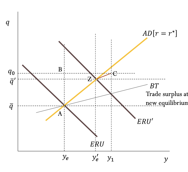
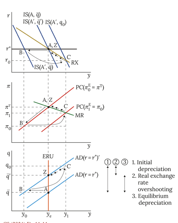
positive supply shock via PS (AD/ERU)

The positive supply shock

raises equilibrium output and

leads to a depreciated

equilibrium exchange rate.

During the period of policy

action, r<r∗. The exchange

rate overshoots. The economy

is off the AD curve. For given

q, output is above where it

would be if r=r∗. For given

output, q is less depreciated

than it would be if r=r∗

(the lower net exports

balancing the higher

investment, compared to a

situation where the economy

was on the AD curve).

positive demand shock policy response(IS/RX)

The shock is a permanent rise in

autonomous expenditure from A to

A’. When ERU is downward sloping

(but not when it is vertical), a permanent

demand shock leads to a change in y𝑒.

The monetary policymaker forecasts PC and

the new RX curve and chooses interest rate

r0 to generate the negative output gap

recommended by next period’s PC and the

MR corresponding to the new equilibrium

output, aiming to get the inflation back to

target at the new equilibrium output.

r0>r* so the exchange rate overshoots.

IS continues to shift as q gradually depreciates from q0 to new equilibrium level qbarprime

positive demand shock policy response(PC/MR)

The central bank forecasts the

new MR curve and next period’s

Phillips curve, which will

correspond to new equilibrium

output and the period-0 inflation

rate the CB forecasts will result

from the shock. The central bank

chooses a (negative) output gap

y1-y 𝑒’ corresponding to that

MR curve and that

adaptive-expectations PC that

reflects inflation expectations

after the shock, pi0,ye’

In subsequent periods, inflation

expectations adjust, the central

bank modifies the interest rate

accordingly, and the economy

returns gradually to the inflation

target at the new equilibrium

level of output.

positive demand shock policy response(WS/PS)

The exchange rate is

appreciated at the new

equilibrium 𝑊/Pc

rises for given W/P, so PS shifts up.

q overshoots, so during the

adjustment period PS rises

above its final level PS’ then

gradually falls back to PS’

as q gradually depreciates

to reach its new equilibrium

value (this adjustment is not

shown).

N0 and N1 are employment

levels corresponding to y0

and y1, where there is

inflationary and disinflationary

pressure, respectively. N0

reflects the situation following

the shock, and N1 corresponds

to the higher unemployment

level after the monetary policy

response.

positive demand shock policy response(BT/ERU)

AD shifts to AD’. CB raises rates, and exchange rate appreciates, r0>r* so exchange rate overshoots to q0, q then gradually deprecates to qbarprime as we return to r=r* on AD.

perm negative demand shock via vert eru

Negative demand shock: AD shifts left

Policy responds with an interest rate

reduction so r<r*

The real exchange rate overshoots: the

initial depreciation jump (qbar to q0) is greater

than the equilibrium depreciation (qbar to qbarprime ).

At C, the real exchange rate q0 is expected to appreciate over the period to qbarprime since r<r* (UIP)

C is off the AD curve since r not equal r*. C is to the right of AD as the lower r<r* results in a higher off-equilibrium value of y for any given value of q

temp positive demand shock w policy response (IS/RX)

The shock is a temporary rise in

business confidence, which is reversed after 1 period. y𝑒 is the same before and after the

shock. The RX curve remains

unchanged.

The monetary policymaker forecasts PC

and chooses interest rate r0 to generate

the negative output gap recommended

by next period’s PC and the unchanged

MR, aiming to get the inflation back to

target at the existing equilibrium

output.

r0>r* so the exchange rate

overshoots.

IS continues to shift as q gradually

depreciates from q0 to unchanged equilibrium level qbar.

temp positive demand shock w policy response (PC/MR)

The central bank forecasts next

period’s Phillips curve, which

will correspond, at the original

equilibrium output, to the

period-0 inflation rate the CB

forecasts will result from the

shock. The central bank uses the

unchanged MR curve and that

forecasted adaptive-expectations

PC which reflects inflation

expectations after the shock, (PC pi0,ye) to choose

(negative) output gap y1-y𝑒.

In subsequent periods, inflation

expectations adjust, the central

bank modifies the interest rate

accordingly, and the economy

returns gradually to the inflation

target at the unchanged

equilibrium level of output.

temp positive demand shock w policy response (PS/WS)

The exchange rate is

appreciated while 𝑟 > 𝑟∗. q

overshoots. Import prices fall

and 𝑊/𝑃𝐶 rises for given 𝑊/𝑃 , so PS

is elevated for the duration of

the policy action: it rises to

𝑃𝑆′ then gradually falls back

to its original level as 𝑞

gradually depreciates back to

its unchanged equilibrium

value (this adjustment is not

shown).

𝑁0 and 𝑁1 are employment

levels corresponding to 𝑦0

and 𝑦1, where there is

inflationary and disinflationary

pressure, respectively. 𝑁0

reflects the situation following

the shock, and 𝑁1 corresponds

to the higher unemployment

level after the monetary policy

response.

temp positive demand shock w policy response (BT/ERU)

The temporary positive

demand shock elicits a policy

response of r>r∗. The

exchange rate responds, and

overshoots. The economy is

off the AD curve.

For given q, output is below

where it would be if r=r∗

For given output, q is more

depreciated than it would be

if r=r∗ (the higher net

exports balancing the lower

investment arising from r>r∗, compared to on the AD

curve).

The BT curve does not shift:

trade remains balanced.

external trade shock policy response (BT/ERU)

A terms of trade shock

shifts the BT and AD

curves. It can be

represented

diagrammatically in a

very similar way to a

demand shock, the

difference being that BT

also shifts (down/right).

The shift in BT is such

that trade is balanced at

the intersection of the

original output level

y𝑒 and new AD curve.

This point represents the

exchange rate at which

appreciation would

reduce net exports to an

extent that exactly

matches the increase in

net exports resulting

from the external trade

shock. otherwise same as demand shock

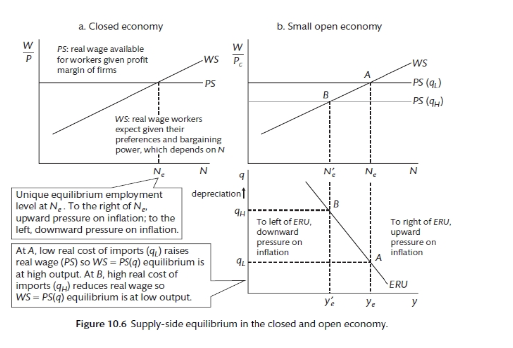
workers care about real consumption vs don’t

In the diagram below, at the WS-PS(𝑞𝐿) intersection: Low import prices raise the real consumption wage so more workers will offer themselves for employment at that wage (point ‘A’). A depreciation would reduce the real consumption wage and employment (point ‘B’).

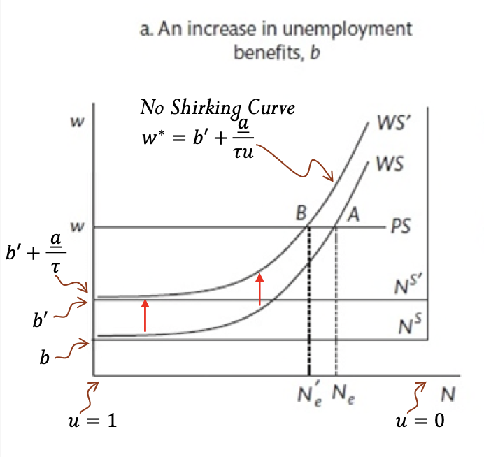
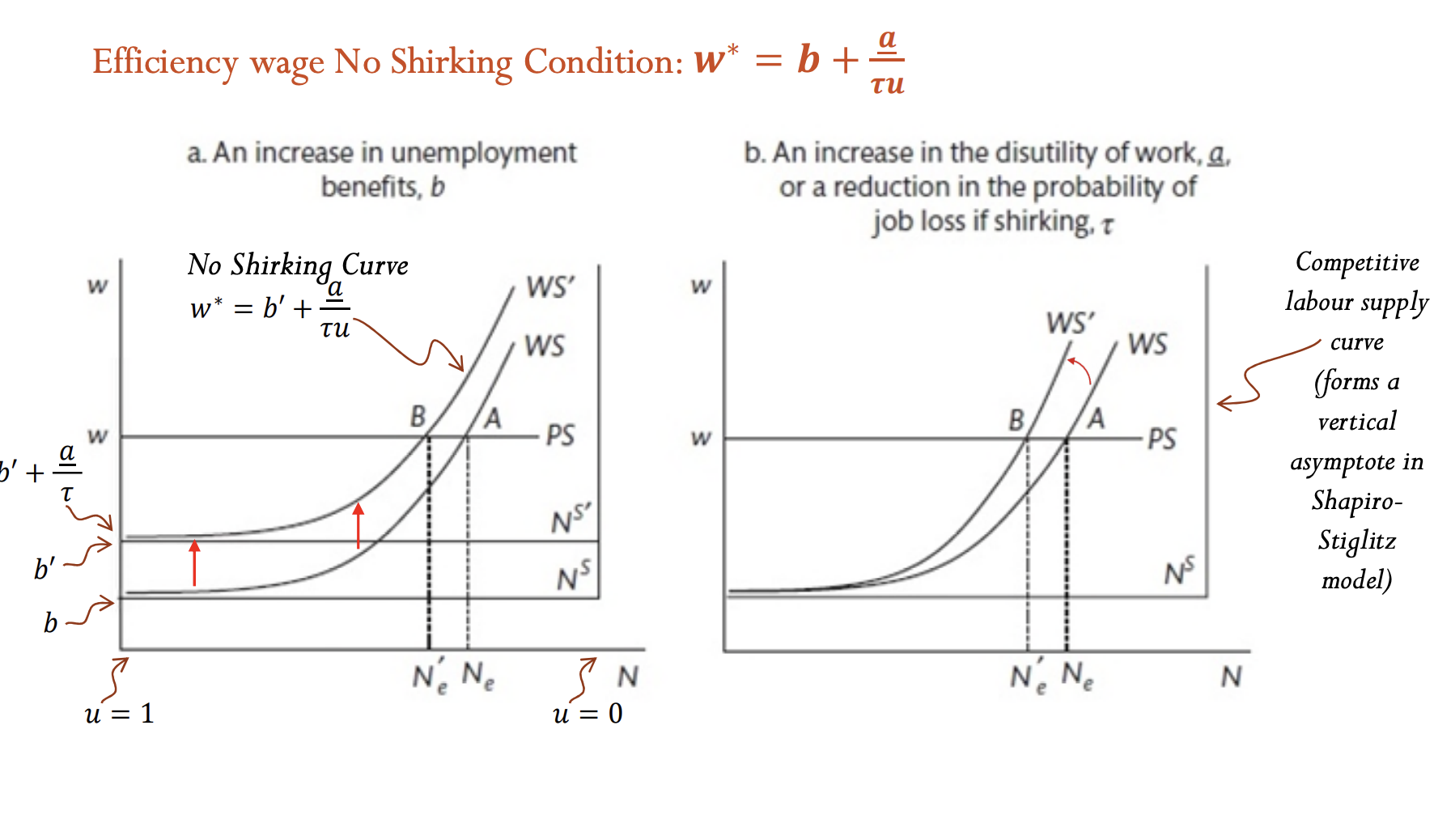
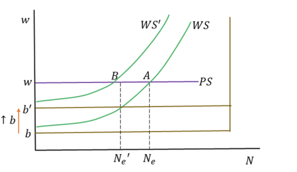
efficiency wage WS/PS model unemployment benefit increase

An increase in b shifts WS upwards since it reduces the cost of shirking and necessitates a higher w* to induce effort. the

moves from ‘A’ to ‘B’.

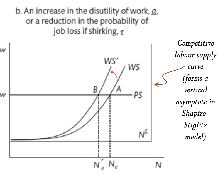
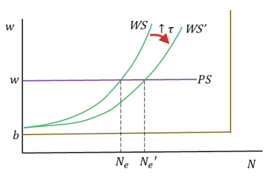
efficiency wage WS/PS model increase in the disutility of work (a↑) or a reduction in the probability of job loss from shirking (tau ↓)

increases the slope of the WS; A higher w* has to be paid to induce effort, and this increases equilibrium unemployment.

efficiency wage WS/PS model Increase 𝜏 (to increase the probability of detection of shirking) by raising the extent of monitoring, or reduce the cost of monitoring.

• In accordance with the multiplicative interaction of 𝜏 and 𝑢 in the efficiency wage expression, a higher 𝜏 increases the extent to which a given change in the unemployment rate 𝑢 affects 𝑤∗. The no-shirking curve will pivot clockwise, leading to a lower equilibrium unemployment rate.

efficiency wage WS/PS modelReduce unemployment benefit 𝑏.

• Reduced unemployment benefit will lower the value of unemployment, making it more attractive to keep a job and thus deterring shirking, for a given wage and probability of detection.

As a result,

• 𝑏+𝑎/𝜏 is the intercept of the no-shirking condition (since at this point 𝑢=1). A rise in 𝑏 shifts the no-shirking curve upwards, leading to a lower equilibrium unemployment rate.

Shapiro Stigiltz one shot game

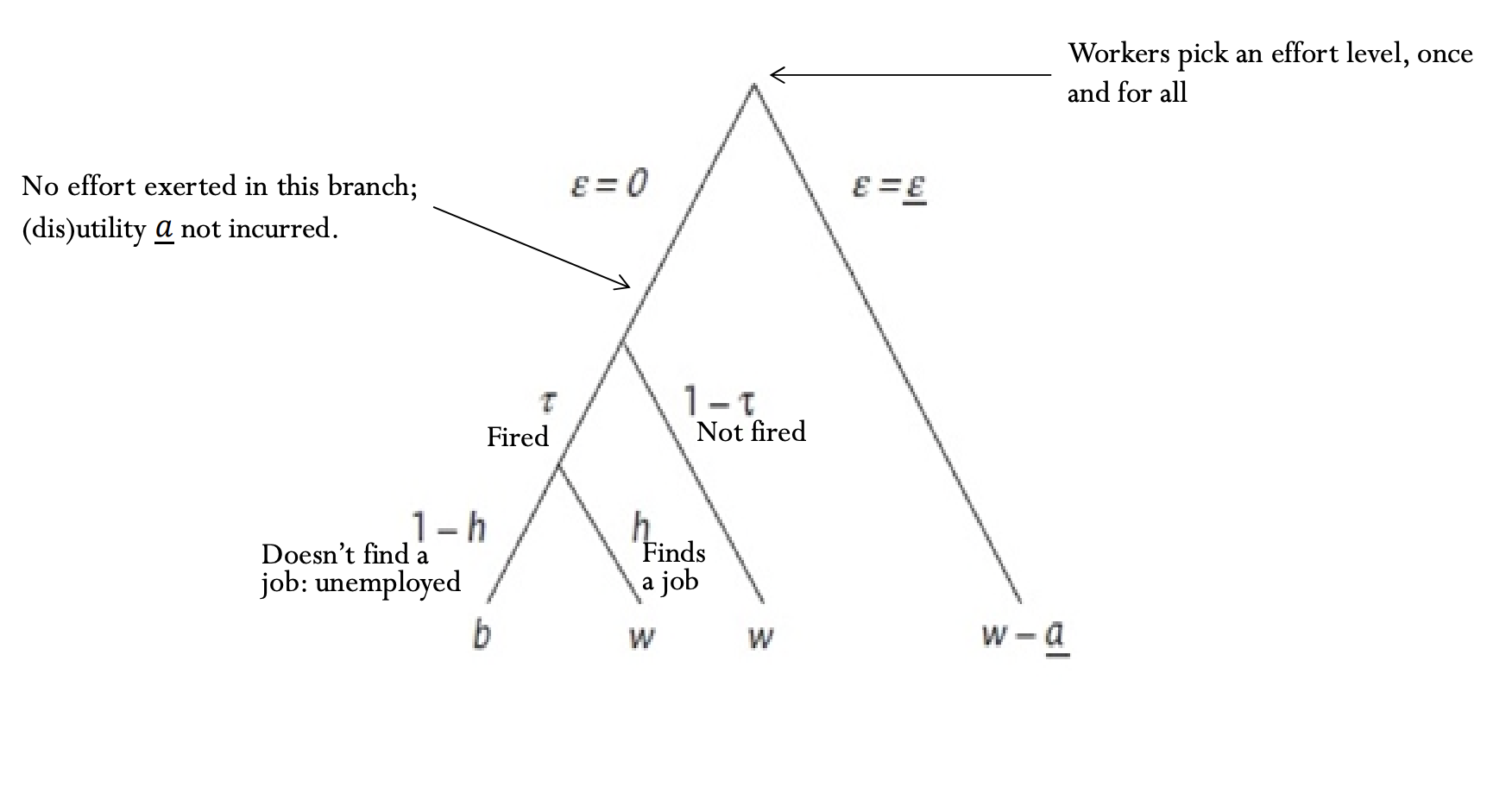
efficiency wage with no shirking conditions. for increase in unemployment benefits, b, and an increase in disutlity of work a or reduction in prob of detecting shriking Tau.

distinguish the shift in WS from a change in b versus the increase in slope due to rise in ‘a’ or reduction in Tau.

also note improving work conditions (lowering a) or lowering benefits (b) or harsher monitoring of work effort (increase Tau) can reduce unemployment