FW 453 Exam II Flashcards

Why estimate population?

• Management and conservation: understand population status, predict and evaluate management consequence/outcomes

• Science: evaluate pop status and change via environmental change

What are the main challenges of estimation?

• sources of error:

  • spatial variation

  • detection probability

• is your pop “closed” or “open”?

• Also, the methods we use must be relevant to the scale we want to estimate at!

  • pop, landscape, community

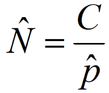
formula for detection probability

N^ = C/p^

(inferences (^) about N require inferences about p)

census

detection probability equals 1 and we count ALL individuals

index

• the count represents some number equal to, or less than, the true number of individuals present

  • detection probability constant but <1

estimate

• a measure of a state variable or vital rate based on a sample of observations

  • typically simultaneously estimates detection probability

Estimation examples in practice

• distance sampling

• capture-mark-recapture

• occupancy modeling

What is distance sampling?

• widely used method for estimating abundance and density (population size/area)

• robust and very popular methodology

  • addresses imperfect detection

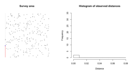
• samples (typically lines or point) are conducted such that objects (e.g. animals, nests, dens, etc) are detected from the sample

• auxiliary info is taken (distances to objects)

  • allows estimation of detection probability as a function of distance to the observer

Distance Sampling Types

• line transects

• point transects

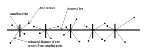
Line Transects

• sample unit is a line of length L placed at a location in the study area

• observer moves along transect recording all individuals detected and their perpendicular distance to transect

• count only objects observed from the line

Assumptions of distance sampling with line transects

1. animals directly on the line are always detected

2. animals are detected at their initial location (no movement response)

3. distances are measured accurately

4. transect lines are placed randomly

5. observation of animals are independent from each other

6. there are sufficient samples to estimate the detection function

Distance sampling with line transects

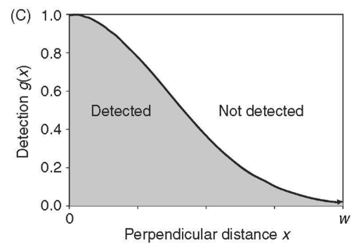
• when detection is not perfect, then we must determine the area sampled in order to estimate density

• D ̂=  n/(2Lμ ̂ )

• •μ ̂  is the “effective half width” of the survey
  – Note: when detection is perfect μ ̂=w

Note that w in strip sampling is set by the user, here, the mew must be estimated!

Violation of independence: clusters

• animals may be in groups

  • objects in groups are not independent

    • treat cluster as the object of detection

• estimating density of clusters

  • need mean cluster size (and variance)

  • need to account for variation in detection (larger clusters more likely to be detected)

How to estimate μ (effective half width of the survey, which is equal to w when detection is perfect)

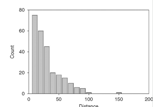
• based on observed frequency distribution, f(x)

• the relative frequency at which distances x from the centerline occur in the sample data

• convert to a probability density function

What is f(x) in distance sampling line transects?

• f(x) is the observed distribution

  • probability of observing an animal at distance x, given that the animal is present and detected somewhere on the transect

What is g(x) in distance sampling line transects?

• g(x) is the detection function

  • probability of detecting an animal, given that it is at distance x from the centerline

Where does μ come in with graphs?

• f(x) = g(x) / μ

• this makes f(x) a probability density function

  • these are easy to work with for estimation problems

There is a relationship between the detection function and the histogram of count data and that relationship is a function of the effective half width of the survey

Estimation of distance function

• f(x) = g(x) / μ

• first assumption: we detect objects on the line 100% of the time

  • g(0) = 1

  • f(0) = 1/μ

  • μ ̂=1/(f ̂(0))

• If we can estimate f(X), and evaluate at x=0, then we can estimate μ

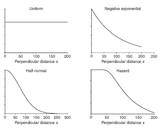
• How do we select a model for f(x)?

• How do we use sample data to estimate f(0)?

Model for f(x)

• Key function is a basic shape for the detection data that describes the way the detection changes as a function of increasing distance from the center line

• We will let Program Distance fit the functions and we will use AIC to determine which is the best model for our specific data (we’ll do this in lab)

How do we use sample data to estimate f(0)?

• after we use program distance to fit a key function to our data, it will use statistical methods to:

  • estimate f(0)

  • which will allow estimation of μ

  • which will allow estimation of density

Why do we add covariates to the model?

The model fit is often poor without the addition of covariates that are likely to influence detection probability

• homogenous bias (observer bias)

• temporal bias (weather/other conditions of survey)

series adjustments (i.e. covariates) are added to improve the model fit like…

f(x) = key(x)[1+series(x)]

• (VIS = visibility; poor/fair (e.g., glare, light fog or rain) or excellent; LIGHT = light conditions; overcast, mostly cloudy, or partly cloudy/clear). ESW = Effective strip width
  (meters). p = Detection probability. ^NN = Abundance estimate. Goodness of Fit metrics: C-S = Chi-squared; K-S = Kolmogorov-Smirnov; C-vM = Crame´r-von Mises

N<

estimated abundance

p<

estimated detection probability

Distance sampling of polar bears

• line transect aerial survey to estimate abundance

• compared against satellite-derived surveys which estimated abundance using capture-recapture

• clouds are factors that may hamper detection

• water conditions are factors that may hamper detection of bears. foam accumulating along edges of water could be confusing

Point Transect Sampling

• establish k points to sample, n observations are recorded at each point

• a point is placed in the study area

• observer spends a predetermined amount of time at the point attempting to detect individuals

• the count of individuals is recorded as well the distance of each from the observer

Density estimation

• D ̂=n/(kπw^2 )

  • k is the number of points surveyed

  • n is the number of animals detected

  • w is the radius of the circle and we assume detection probability is perfect out to this distance

kπw²

the cumulative area of the k points surveyed

the frequency of observations at each radial distance (r)

f(r)

• analogous to f(x)

h(r)= g(x) detection function for ___

radial distances r

• we use the same method: fit a key function to f(r)

• assumptions are the same as for line transects

D ̂=(nf′(0))/2kπ

• instead of using f(0) for density estimation, we use f’(0)

  • f’(r) is the derivative of f(r)

• remember

  • μ ̂=1/(f′(0))

Sampling principles

• What is the objective?

• What is the target population?

• What are the appropriate sampling units?

  • quadrats?

  • point samples?

  • line transects?

3 types of sampling units

• Quadrats

• point samples

• line transects

Comparison of line transects vs. point counts

• line transects

  • typically preferred for mammals

  • cover larger areas more quickly

  • distance estimation when moving may be more difficult

• point counts

  • typically preferred for birds

  • more practical in rough terrain

  • fixed time at each station

  • more time to see or hear

    • especially important for birds in high canopy

  • less area covered to see or hear

    • especially problematic for mammals

Advantages and disadvantages of samplings units—nonrandom placement

• advantages

  • easy to lay out

  • more convenient to sample

• disadvantage

  • do not represent other (off road) habitats

  • road may attract (or repel) animals

Advantages and disadvantages of samplings units—random placement

• advantages

  • valid statistical design

  • represents study area

  • replication allows variance estimation

• disadvantage

  • may be logistically difficult

  • may not work well in heterogeneous study areas

Advantages and disadvantages of stratified sampling

• advantages

  • controls for heterogeneous study area

  • allows estimation of density by strata

  • more precision

• disadvantages

  • more complex design

Takehomes for Strip transects

• Detection is assumed constant across the transect

• Tends to underestimate density

Take homes for line/point transects

• Distances are recorded for each observation

• Detection is modeled as a function of distance

• Effective transect width/point area is modeled based on the detection function

• Density estimates take into account the effective transect width and missed individuals

Variables N, C, and p in detectability meaning

• N= abundance

• C= count statistic

• p = detection probability; P(member of N appears in C)

• C = pN

Inferences about N require inferences about p

N> = C/P>

Lincoln-Petersen Method

• Frederick Lincoln and Gustav Petersen

• Capture, mark and release a sample of individuals from a population

• At a later date, take a second sample

• Proportion marked individuals in the second sample indicates proportion of total pop we sample each time

  • detection probability!

Marking animals for L-P: Batch marking

• Groups of animals are given the same marks

  • i.e., marks are not uniquely identifying, animals are simply either marked or not

• Examples?

• Limitations?

the basic estimate for abundance

• N = n₁n₂/m₂

  • N = abundance

  • n₁ = the number of animals caught and marked at capture occasion 1

  • n₂ = the number of animals caught at capture occasion 2

  • m₂ = the number of marked animals caught at capture occasion 2

What is detection probability (p) under the Lincoln-Petersen model?

p = m₂ / n₂

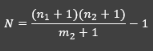
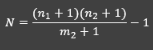
We commonly use an adjusted estimator that is unbiased for small sample sizes:

• N = ((n+1)(n₂+1))/(m₂+1) — 1

• If sample size is small, the LP estimator is biased. For example, what happens if the number of recaptures is zero?

The estimated variance is calculated as:

var(N) = ((n₁+1)(n₂+1)(n₁-m₂)(n₂-m₂)) / ((m₂+1)²(m₂+2)

The approximate 95% Cls are

N ± 1.96 sqrt(var(N))

Rabbit abundance in Oregon example

• Rabbits were captured in central Oregon and marked by dying their tails and hind legs with color

• 87 were initially captured and marked

  • Live trapping

• 14 were captured a second time, of which 7 were marked

  • Drive counts

• Based on the results, we can set up the problem with:

  • n1 = 87

  • n2 = 14

  • m2 = 7

• Then we use the adjusted L-P to find our estimate of N

  • 𝑁=((𝑛_1+1)(𝑛_2+1))/(𝑚_2+1)−1= (87+1)(14+1)/(7+1) −1=164

• We can also calculate the variance of N and the approximate 95% Cl

  • var(N) = 1283.33

• The 05% Cl is (93.8 to 234.2)

• Overall detection probability = 0.5

  • p = m2/n2 = 7/15 = 0.5

• But they used 2 diff methods so we can see which had the higher detection probability

  • live trapping: p = 87/164 = 0.53

  • drive counts: p = 14/164 = 0.09

  • because of two different methods, our estimate of p is not very good, we need to estimate p separately for each method. Live trapping has much higher detection probability so is a better method for estimating N in this population.

  • The variation in capture probabilities between occasions is allowed in L-P!

• Assumptions:

  • the pop is closed

  • all animals have the same probability of being caught within an occasion

    • first occasion capture does not affect second

  • there is no tag loss or other loss of marks

  • Catching an animal does not affect its probability of capture on subsequent occasions. Marks are accurately recorded.

Closed population

• Abundance is constant during the study

• No gains or losses (i.e., births, deaths, immigration, emigration)

• Most of the models we do, will make this assumption

Open population

• Abundance may be constant or change

• Subject to gains and losses

• We can estimate survival, recruitment, movement, etc. if the sampling is well designed

Assumption of equal detection

• All animals have the same probability of being caught within an occasion

• What might impact this assumption?

  • i.e. when might it be violated?

  • Sampling technique
    Gear
    Time of year
    Home range size differences between sexes

Violations of Equal Detection

• Trap happy

  • Animals are more likely to show up as recaptures than would be predicted

  • p will increase, N will decrease

• Trap shy

  • Animals are less likely to show up as recaptures than would be predicted

  • p will decrease, N will increase

Individual Marking

• Marking animals individually gives us extra information

  • Can relax some assumptions of Lincoln - Petersen

• Allows use of more complex models with multiple samples (occasions)

  • Allows us to account for variation in capture probabilities!

Multiple sample CMR

• 2 or more occasions

• Advantages

  • more data to estimate N=more precision

  • avoid some assumptions of LP

    • all animals NO LONGER have the same probability of capture

    • probability of capture can be affected by previous experience of capture

M0 model

• constant detection probability (p)

  • Over time, individuals, behavior

Mt model

• only time effects

  • – L-P is a special case with k=2

Mb

• only behavioral effects

  • Trap happy or shy

Mh

• individual effects

  • Heterogeneity in capture probabilities

Combination of model effects

Mth, Mtb, Mbh, etc

What does 00000 mean in multiple sample CMR?

not captured at all

𝜔

individual encounter histories

encounter history

• An encounter history tells us whether an individual has been captured/detected during each sampling occasion

• Written as a 1 if an individual is encountered and a 0 otherwise

• For 2 time occasions:

  • 01: not captured first time, captured second sample

  • 10: captured, not captured

  • 11: captured, captured

  • 00: not captured at all

Using the encounter history we can summarize the data into totals for each category:

• 𝑋10 number caught on the first occasion but not the second

• 𝑋01 number caught on the second occasion but not the first

• 𝑋11 number caught on both occasions

• 𝑋00 number never caught

• 𝑟 = 𝑋10 + 𝑋01 + 𝑋11 total number of different animals caught over the study

• Total of all is our population size, so why not just add up all 4 categories?

How do encounter histories help us estimate?

• We will calculate the probability of each unique combination of 1s and 0s (Pr(𝜔))

• Using Pr(𝜔) and the observed frequency of each unique combination of 1s and 0s (𝑋𝜔), we can obtain estimates of capture and recapture probabilities

  • Via maximum likelihood, which we will leave to Program MARK

• With this information, we can then estimate 𝑁 by what is basically an extension of the L-P estimator

𝑝𝑖𝑗

capture probability for each individual i at each time j

𝑐𝑖𝑗

recapture probability for each individual i at each time j

If we assume capture probability is constant over time then…

𝑝𝑖𝑗 = 𝑝𝑖 and 𝑐𝑖𝑗 = 𝑝𝑖

𝑘

the number of capture/recapture occasions during the study

Review of basic probability rules

• Rule 1: Probabilities must be between 0 and 1

• Rule 2: The sum of the probabilities for all possible outcomes of an event must equal 1

• Rule 3: The probability that an event does not occur is 1 minus the probability that it does occur.

• Rule 4: The probability that two events both occur together is found by multiplying the probabilities that they occur alone

• Rule 5: If two events CANNOT occur together, the probability of them both occurring is found by adding their probabilities

Model M0 assumes…

• constant and homogenous p

  • i.e., capture probability is constant across time and individual

  • Therefore, 𝑝𝑖𝑗= 𝑝 and 𝑐𝑖𝑗=𝑝

  • It has 2 parameters: N and p

Say we have:

• 𝜔 = 101

what is Pr(𝜔) under m0 model?

Pr(𝜔) = 𝑝(1 − 𝑝)𝑝

How about:

• 𝜔 = 000001

(what formula under M0?)

• Pr(𝜔) = (1 − 𝑝)(1 − 𝑝)(1 − 𝑝)(1 − 𝑝)(1 − 𝑝) 𝑝

• which can be written as:

  • Pr(𝜔) = (1 − 𝑝)5𝑝

IF 𝜔 = 000000…

under model M0, Pr(𝜔) =

Pr(𝜔) = (1 − 𝑝)6

Calculating Pr(𝜔) under Model Mt

• 𝑝𝑖𝑗 = 𝑝𝑗 and 𝑐𝑖𝑗 = 𝑝𝑗

• So model parameters are N and p1…pk

• Now, say we have

  • 𝜔 = 101

  • "Pr(𝜔) = 𝑝1(1 − 𝑝2)𝑝3"

• If we have k=6 occasions, then we might have

  • 𝜔 = 101011

  • Pr(𝜔) = 𝑝1(1 − 𝑝2)𝑝3(1 − 𝑝4)𝑝5𝑝6

• How about:

  • 𝜔 = 000001

  • Pr(𝜔) = (1 − 𝑝1)(1 − 𝑝2)(1 − 𝑝3)(1 − 𝑝4)(1 − 𝑝5) 𝑝6

Calculating Pr(𝜔) under Model Mb

• If we assume capture probability varies after the first capture, but is constant otherwise, then

  • 𝑝𝑖𝑗 = 𝑝 and 𝑐𝑖𝑗 = 𝑐

• For our previous encounter history

  • 𝜔 = 101011

  • Pr(𝜔) = 𝑝(1 − 𝑐)𝑐(1 − 𝑐)𝑐𝑐

• We can reduce this to:

  • Pr(𝜔) = 𝑝(1 − 𝑐)2c3

• How about:

  • 𝜔 = 100001

  • Pr(𝜔) = 𝑝(1 − c)(1 − c)(1 − c)(1 − c) c

Model M_h

• This model allows capture probabilities to vary by animal, due to heterogeneity, but there is no trap response or time variation.

• The parameters in the model are:

  • 𝑁

  • p1…𝑝𝑖 - the capture probability of animal 𝑖

• When might we use this model?

Calculating Pr(𝜔) under Model Mh

• If we have individual effects, the model can get complicated:

  • 𝜔 = 101011

  • Pr(𝜔) = 𝑝𝜔(1 − 𝑝𝜔) 𝑝𝜔(1 − 𝑝𝜔) 𝑝𝜔 𝑝𝜔

• Basically a unique detection probability for each individual

• How about:

  • 𝜔 = 100001

  • Pr(𝜔) = 𝑝𝜔(1 − 𝑝𝜔)(1 − 𝑝𝜔)(1 − 𝑝𝜔)(1 − 𝑝𝜔)𝑝𝜔

What happens when you combine behavioral, time, and individual effects?

• If we have behavioral, time, and individual effects, the model can get very complicated:

  • 𝜔 = 101011

  • Pr(𝜔) = 𝑝𝜔1(1 − 𝑐𝜔2) c𝜔3(1-c𝜔4)𝑐𝜔5𝑐𝜔6

• Basically a unique detection probability and recapture probability for each individual at each time step – difficult to fit without plenty of data!

Estimation for p and c

• We will use a likelihood based approach

  • Use observed frequencies (𝑋𝜔) and (Pr(𝜔))

  • Multinomial likelihood

  • Estimates p and c probabilities

  • Use this information to estimate N!

Variables in model variation in capture probability

• Model variation in capture probability as a function of

  • Time (t)

  • Behavior (b)

  • Individual heterogeneity (h)

  • Combinations (b*t, b*h, etc.)

• Compare models

  • AIC

What is the best way to estimate abundance with 2 samples?

The Lincoln-Petersen method

Basic multi-sample CMR model types

• M_0 — constant capture probability (p)

  • over time, individuals, behavior

• M_t — only time effects

  • L-P is a special case with k=2

• M_b — only behavioral effects

  • trap happy or shy

• M_h — individual effects

  • heterogeneity in capture probabilities

• combinations of effects (M_th, M_tb, M_bh, etc)

Cormack-Jolly-Seber Model

• apparent survival (cannot differentiate death from emigration)

• capture probability—but cannot estimate N!

Jolly-Seber model

• estimation of survival and recruitment (theoretically)

• can estimate N with strong assumptions but difficult to fit

Pollock’s robust design model

• combines closed and open modes, N, survival and recruitment among other things

• incredible amount of flexibility

p_j

capture probability for at each time j

• if we assume capture probability is constant over time then pj = p

φ𝑗

apparent survival for at each time j

• if we assume apparent survival is constant over time, then φ𝑗 = φ

Why is there no N in the Cormack-Jolly-Seber model?

we are not interested in abundance, only apparent survival

Closed population vs open population diagrams

In the closed population, animals don’t leave, so there is just the “marked and release” tab with “captured” (p) and “not captured” (1-p) counts. But with open populatoin, we start with the “marked and released” tab which splits into “alive” (𝜙) and “dead/emigrated" (1-𝜙),” and “alive” is split into “captured” (p) and “not captured” (1-p)

Types of CJS models

M₀0

M_t0

M₀t

M_tt

CJS model M₀0

•  constant detection and survival

  • 2 parameters: 𝑝 and 𝜙

CJS model M_t0

• time specific detection, constant survival

  • Separate p for each time period and a single 𝜙

CJS model M₀t

• constant detection, time specific survival

  • Separate 𝜙 for each time period and a single p

CJS model M_tt

• detection and survival are time specific

  • Separate 𝜙 AND p for each time period

CJS M_00 — calculating Pr(𝜔)

• Now we have p and 𝜙, the detection probability and survival rate respectively

  • 𝜔=101

  • Pr⁡(𝜔)=𝜙(1−𝑝)𝜙𝑝

• We condition on the animal being captured in time 1. So we don’t estimate p or 𝜙 for time 1. We ONLY consider animals with a 1 for the first period

• This 𝜙 is the probability the animal survives from the PREVIOUS time (Time 1)

• We know it (the 101) survived since we captured it in Time 3!

• We know this animal survived to time 3, therefore it was alive during Time 2 but not recaptured (1−𝑝)

• This animal was recaptured in Time 3, therefore it was both alive and captured (𝜙𝑝)

• These quickly get more complicated because we not only have to keep track of whether an animal is detected in a given period, but whether they were detected in subsequent periods

• This gives us the information we need about survival to calculate P(𝜔)

Given the follow capture histories, what are the probabilities under M₀0?

• 111

• 110

• 101

• 100

• 𝜙p𝜙p

  • ignore the first 1 and only consider the next two 1s. Each one has 𝜙p

• 𝜙p(1-𝜙p)

  • Ignore first one and consider the 0. The second 1 gets 𝜙p but this time we also multiply by (1-𝜙p) because it was not recaptured (0)

• 𝜙(1-p)𝜙p

  • Ignore first 1. Now we have 0 and 1. The 0 indicates it wasn’t recaptured, so we do 𝜙(1-p). But then it was recaptured so it gets a 𝜙p

• (1-𝜙) + 𝜙(1-p)(1-𝜙p)

  • Ignore the first 1. We only have 2 0s. So, we have (1-𝜙) + 𝜙(1-p)(1-𝜙p). The animal was never recaptured, we now have 2 possibilities (last row).

note: We condition on the animal being captured in time 1. So we don’t estimate p or 𝜙 for time 1. We ONLY consider animals with a 1 for the first period

Assumptions of the CJS

• Homogeneity of capture and survival probabilities for the marked animals within each sample occasion and group

  • Individual heterogeneity can also be modeled similar to model M_h but is pretty complex

• Instantaneous recapture and release of animals

  • Keep trapping short relative to the interval between trap occasions

• All emigration from the study area is permanent (no temporary emigration)

Issues of Jolly-Seber model

• Estimating the proportion of animals marked on each occasion is tricky and estimates of N may be biased as a result

• As a result, estimating recruitment is difficult and models rarely converge

• Estimates of abundance and recruitment are not robust to heterogeneity in capture probabilities

Difference between CJS and JS models

• CJS models

  • Estimate survival and capture probability

  • Condition on marked individuals

• JS models

  • Estimate survival, capture probability, abundance and recruitment

  • Must estimate the proportion of individuals in the population at each time step

    • Tricky

  • No heterogeneity in capture probabilities allowed!