DAPAB W4L2/W4D3: Mixed model using all relationships and ReML

Main traditional reasons for mixed model

Non-independence/estimate the fixed effects accounting for all the noise (P-values, SE)

Estimating variance components: reasons for ReML
ANOVA does not work for VCE with unbalanced data

Use ReML

Traditional reasons for mixed models and ReML

Recovery of inter-block information with incomplete blocks

Use ranodm block effects for identifiability of fixed effects of interest

In animal breeding, interest is in the

random breeding values → BLUPs

and in the aditive genetic ariance in non-designed populations (dismgaA) → ReML

The fixed effects merely serve as correction factors (herd, year, season age)

The BLUEs of fixed effects are usually not of main interest in animal breeding

Mixed models and ReML in animal breeing

Interest is in the random effects

• Breeding values

• Gene effects

• → need the variance components

Unbalanced data

• unequal family sizes

General pedigrees

• Related sires and dsams

• Any type of relatedness

• Use all family information, e.g. all dutch cows

Non-random samples

• selection of superior individuals

Non-ranodm mating

Include genomic informaiton

• Genomic breeding values

  • GWAS

Mixed models and ReML in plant breeding

Interest is often in the fixed effects

Unbalanced data (e..g incomplete blocks)

Include genomic information

• GWAS

Fixed or random

Simplicity

• Fixed effects are simpler, models converge better (least squared instead of ReML)

Conceptual reasons

• Is your model term a random sample of a population?

• Sex effect: NO, there are only two sexes→ sex is fixed

• Pen: YES, there could be many different pens → pen is random

Avoid false significance in hypothesis testing (avoid too small P-values)

• For example: does sex affect body weight of pigs

  • Include sufficient noise in the model to avoid false significance

  • Test for sex effect: fit pen, batch etc as random effects

Avoid overstimation of effects (BLUPS)

• Random effects (BLUPs) get shrinkage → estimates are conservative

• Fixed effects (BLUEs) get no shrinkage → suffer from winners curse

• Fixed effects are greedy

• Fixed effects absorb too much varaition when classes are small

Partial confounding, fixed effects have priority over random effects

• Recovery inter-block information → blocks must be random

  • Fixed variety effect has priority over the random block effect

  • So inter=block info can be utilized

Relationships/correlations

• Random effects can be correlated (e.g. related animals)

• → genetic effects are treated as random

Real life: why did we not simply skip ANOVA

ANOVA requires many assumptions that never hold

• Real data are never balnaced

• Sires and dams tend to be related

• Preselection is common in breeding populations

ANOVA shows where the information comes from → helps understanding of what we do

ReML is way more powerful, but we do not see where the inforamtion comes from

For balanced designs; ANOVA and ReML are

Equivalent

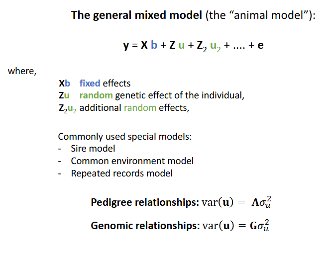
The general mixed model for genetic analysis

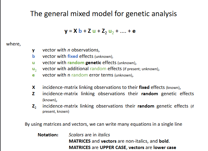
The general mixed model for genetic analysis

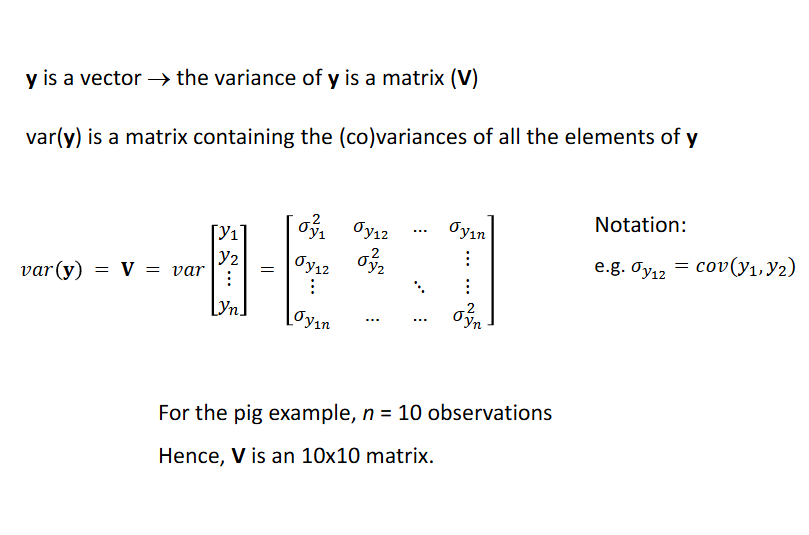
Y is a vector → the variance of y is a matrix V

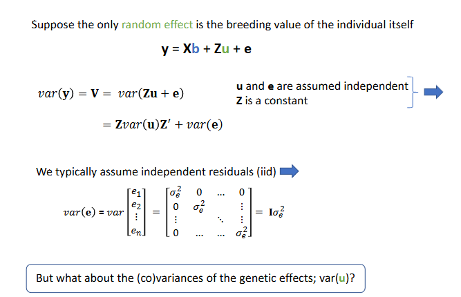
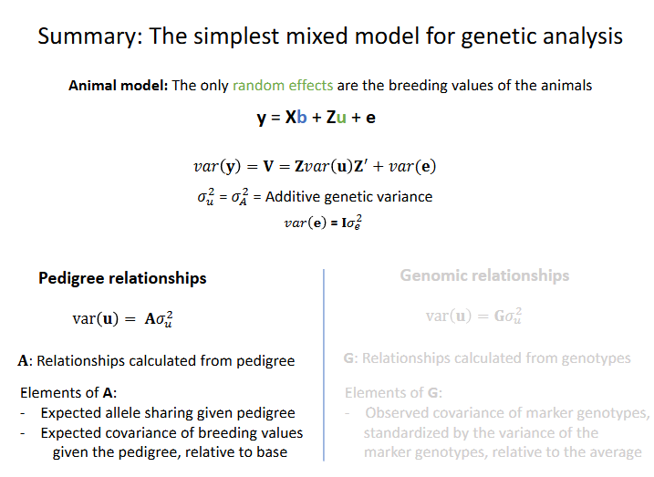
Animal MOdel: the simplest mixed model for genetic analysis

Residual identical distributed

The u-effects (breeding values) of related animals are

Positively correlated, related animals have similar breeding values

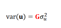
About the (co)variances of the genetic effects, var(u)

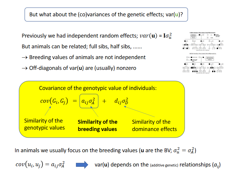
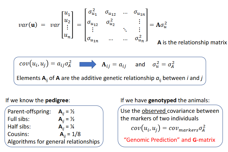
Relationship matrix

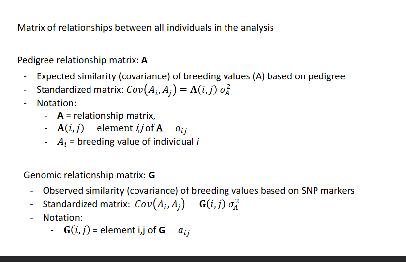
Matrix of relationships between all individuals in the analysis

• Pedigree relationship matrix A

• Genomic relationship matrix G

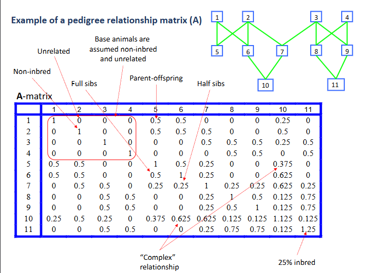
The pedigree relationship matrix A

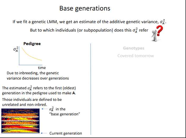
Base generations

Example of a pedigree relationship matrix A

Summary: the simplest mixed model for genetic analysis

Models for special cases

Sire model

Common environmental effects (litter effects)

Repeated records and permanent non-genetic (environmental effects)

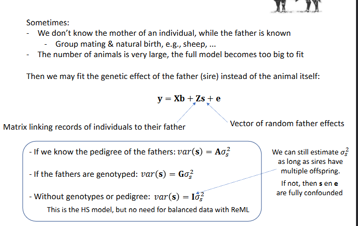
The sire model

Sometimes, we don’t know the mother of an individual, while the father is known (group mating and natural birth, sheep etc). The number of animals is very large, the full model becomes too big to fit

Then we may fit the genetic effect of the father (sire) instead of the animal itself

The sire model - interpretation

Interpretaion

• similar to the half sib model

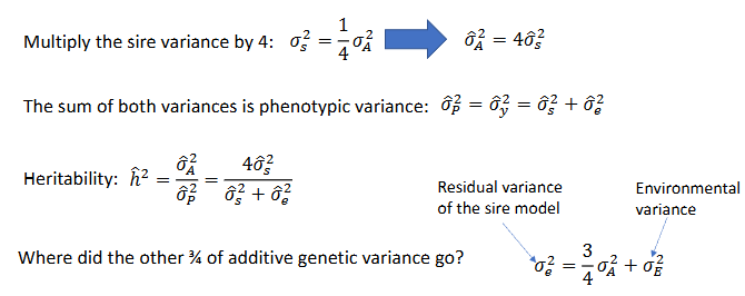
• - Offspring of the same sire are half sibs → var(sire) = cov(half sibs)

• Cov(half-sibs) = 1/4 var(A)

  • The sire variance is an estimate of a quarter of the additive genetic variance

The sire model - assumptions

1. Without genetypes or pedigree: var(s) = Isigmas2

the sires are assumed unrelated

The sires are assumed to be random sample of the population

2. The dams

are assumed to be random sample of the population

unrealted to the sires

mated at random to the sires

each dam contributes a single offspring (No full isbs in the data)

Same assumptions as for the HS design with ANOVA (no need for balanced data)

What would happen if we appply a sire model to a pig population?
pig data contain full sibs

We overestimate heritability

Common environmental effects - piglest born in the same litter

Are full sibs (usually)

Developed in the same uterus

Also receive the ordinary animal model to data on weaning weight: y=Xb+Zu +e

Solution for common environmental effects

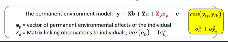
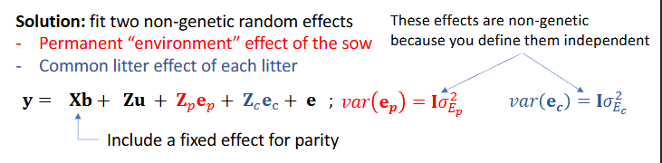
The common environmental model: y=Xb + Xu +ZCec +e

ec: vector of random effects common to litter mates (common environment)

Zc: matrix linking observations on indiviuduals to their birth litter

Litter effects are assumed independent 𝑣𝑎𝑟 𝐞𝒄 = 𝐈𝜎𝐸2
Genetic effects are correlated via the pedigree or genotypes: var(u) = 𝐀𝜎𝐴2

The common litter effect also captures (most of) the dominance variance, therefore we don’t usually fit a separate dominance effect

We can separate litter and genetics when

The sire is not completely confounded with litter, thus HS provide info for simgaA2

The different dams may be related, but their litter effects are independent

• Therefore the ReML likelihood depends on sigmaA2 and we can estiamte it

• With FSHS ANOVA we could not separate genetic and non-genetic dam effects

But

• The full-sib covariance is completely confounded with litter, thus litter effects reduce precision (and power) to estimate SigmaA2

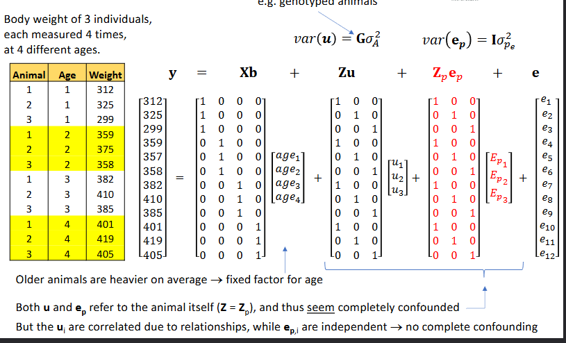
Repeated records - some traits we may record multiple times on the same animal

Body weight at different ages, milk yield each week or month, litter size in different parities

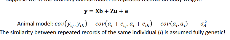
Suppose we fit the ordinary model to repeated records on body weight

The similarity between repeated records of the same individual (i) is assumed fully genetic

But what if

• the animal has been sick when it was young, poor nutrition when it was young → permanent environmental effects (developmental effects)

Repeated records - permanent environment model

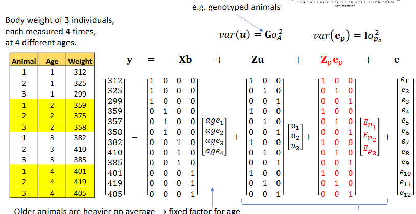
Repeated records - example

Repeated records and common environment

Data consists of the following:

• For each ltiter, we have weaning weight of each piglet

  • Within a ltiter, piglets experience a common environment (Ec)

  • But piglets in different litters are also nursed by the same mother (Ep)

Genetic relationships

Geneomic relationships

replace the pedigree relationship matrix A with the genomic relationship matrix G

→ more powerful than pedigree, similar to pedigree

Genomic relationships and the G-matrix

If we have genotyped the animals:

Use the observaded covariance between the markers of two individuals

cov(ui,uj) = covmarkersSigmaA2

Genomic prediction and G matrix

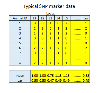
MARKERS = SNP-markers

SNP-markers

m marker loci

Each locus has 2 alleles, e.g. A and T

We count one of the two alleles, say A

Diploids → counts are 0,1 or 2, TT=0, AT and TA are 1, AA=2

p is the frequency of the counted allele - count ~ BIn(n=2,p)

The mean allele count is 2p

The varaince in allele count = 2p(1-p)

Genomic relationships: the observed covariance between markers of animals

The common way to calculate a covariance from a sample

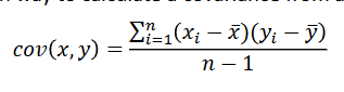
Genomic relationships: the observed covariance between markers of animals

With markers - covariance

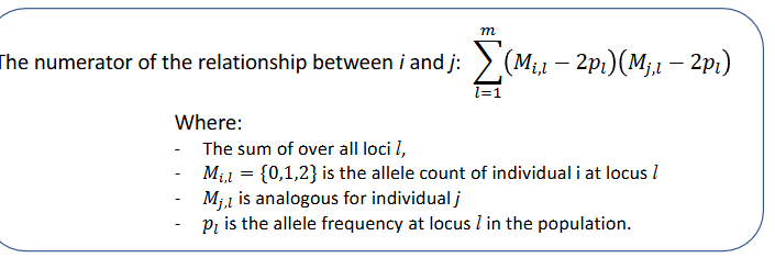
We want the covariance between two individuals, say i an j, due to all the m markers

x and y are the allele counts in the two individuals, with values M = { 0,1,2}

For a specific locus (l), the mean x and y is two times the allele frequency, 𝑥(^-) =y(^-)𝑙 = 2𝑝l

There are many loci, so n -1 = n, ignore the -1

Genomic relationships: the observed covariance btween markes of animals

The numerator of the relationship between i and j

Genomic relationships: the observed convarience between markers of animals

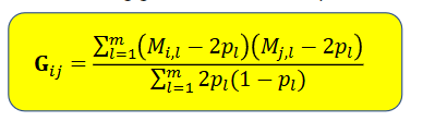
Next, we want to write var(u) as: var(u) = G(sigmau2)

where 𝐆𝜎𝑢2 is a covariance matrix

Hence, G is a standardized covariance matrix

We have to standardize (divide) the covariance by the marker variance

The resulting geomic relationship in yellow

Gij is the similarity of the markers of i and j, measured as a standardized covariance

A and G do not depend on the trait, but only on the

Pedigree (A) or on the genotypes (G)

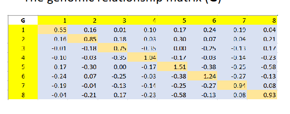
The genomic relationship matrix (G)

Note:

• G has both positive and negative values

• Off-diagnoals Gij: relationships between different individuals

• - positive values → individuals are more similar than average

• negative values → individuals are less similar than average

Diagonal elements Gij: self relationships = 1+ inbreeding coefficient

• smaller than 1 → individual is less inbred (homozygous) than average

• larger than 1 → individuals is more inbred (homozygous) than average

in contrast to the pedigree relatiosnhisp (A), negative relationships and inbreeding can exist

This is because G measures allele sharing, relative to the population aveage

Large sample in HWE: mean off-diagnoals: G(^-)ij = 0, mean diagonal g(^-)ii=1

Base generations

If we fit a genetic LMM, we get an estimate of the addivie genetic variance

BUt to which indivudals or subpopulation does this additive genetic variance refer to

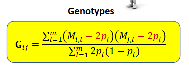
GENOTYPES

In G, we subtract 2p when calculating the covariance → the mean genomic relationship is zero in the pouplation we used to calculate p → with genomic relationships the additive genetic variance refers to the pouplation we used to calculate p, usually htese are the genotyped individuals

Summary - mixed model using all relationships and ReML