Probability for Engineers Final

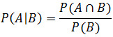
Conditional Probability Formula: P(A|B)

Disjoint

A and B = empty set

Bayes Rule: $P(A|B)$

$$P(A|B) = \frac{P(B|A) \cdot P(A)}{P(B)}$$

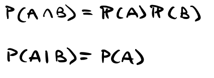
Independence

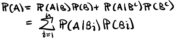
Law of Total Probability

Pairwise Independence

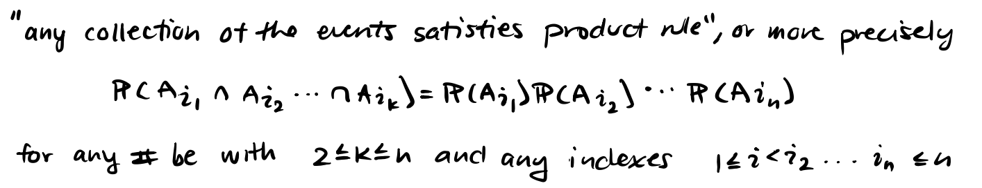
Jointly Independent

How many ways to assign k states to each n things?

With replacement, order

kⁿ

How many ways to list m distinct things out of n?

W/o replacement, ordered

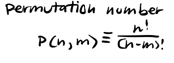
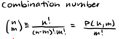
How many ways to fill a bag with m items out of n items?

W/o replacement, unordered

Discrete Random Variable

Finite or countably infinite set of values

Probability Mass Function (PMF) of discrete random var X

Bernoulli: X~Bernoulli(p)

single binary experiment with two possible outcomes: "success" (1) with probability or "failure" (0) with probability

E[X]=p

Var(x)=p(1-p)

Geometric: X~Geometric(p)

Parameter: 0 < p < 1 success probability

Models: # of independent trials until 1st success

E[X] = 1/p

Var(X) = (1-p)/p²

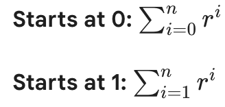
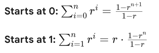
Finite Geometric Series

Binomial: X~Binomial(n,p)

Parameters: p = success prob (0<p<1), n = # trials to be performed

Models: # success from n independent trials, w/ each trial success prob p

E[X] = np

Var(X) = np(1-p)

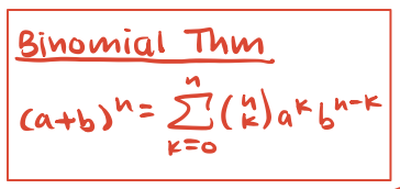
Binomial Theorem

Poisson: X~Poiss(lambda)

Parameter: lambda > 0 (rate parameter)

Models: (A) # arrivals within some unit of time, (B) “Rare events”

E[X] = lambda

Var(X) = lambda

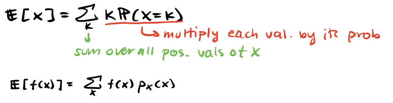
Expected Value: E[X] and E[f(x)]

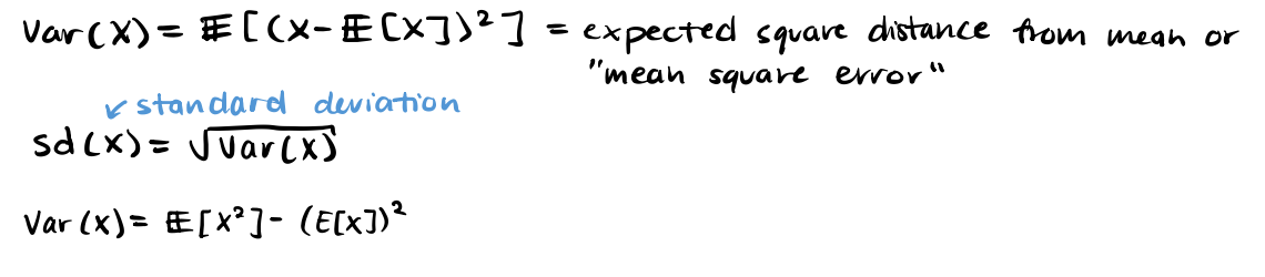
Variance, standard deviation

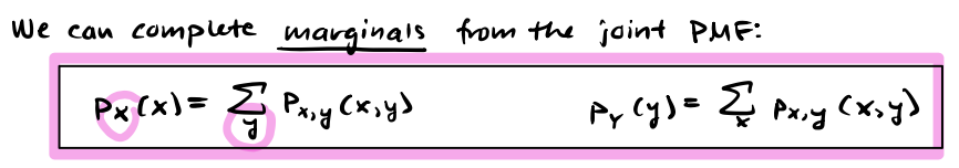
Marginal PMF (discrete)

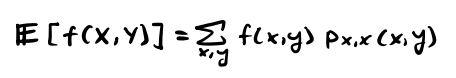
E[f(X,Y)] - Discrete

Linearity of Expectations (Discrete)

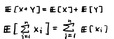
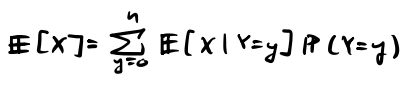
Law of Total Expectation

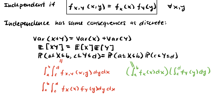
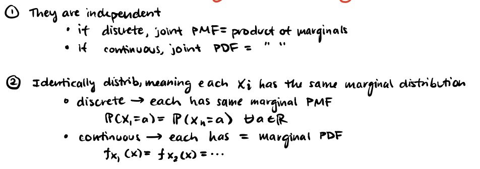
Independence for X, Y

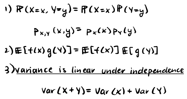
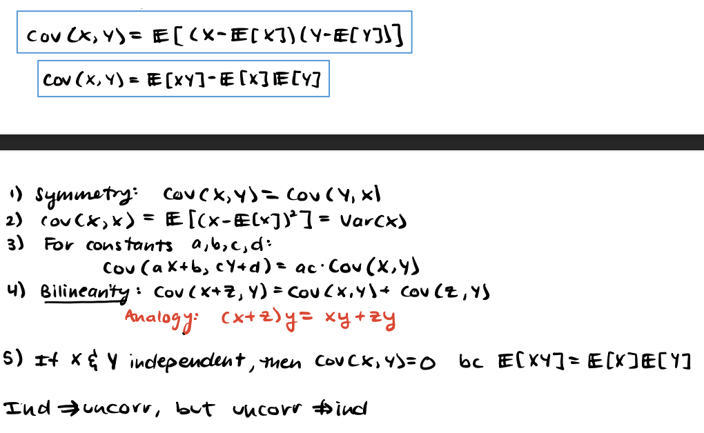
Covariance: Cov(X,Y)

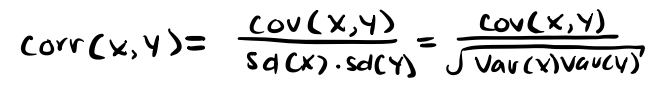
Correlation: Corr(X,Y)

Continuous Random Variables

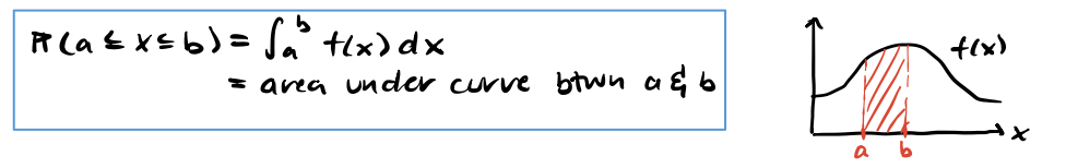
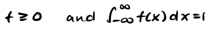
Defining Properties of PDF

Cumulative Distribution Function (CDF)

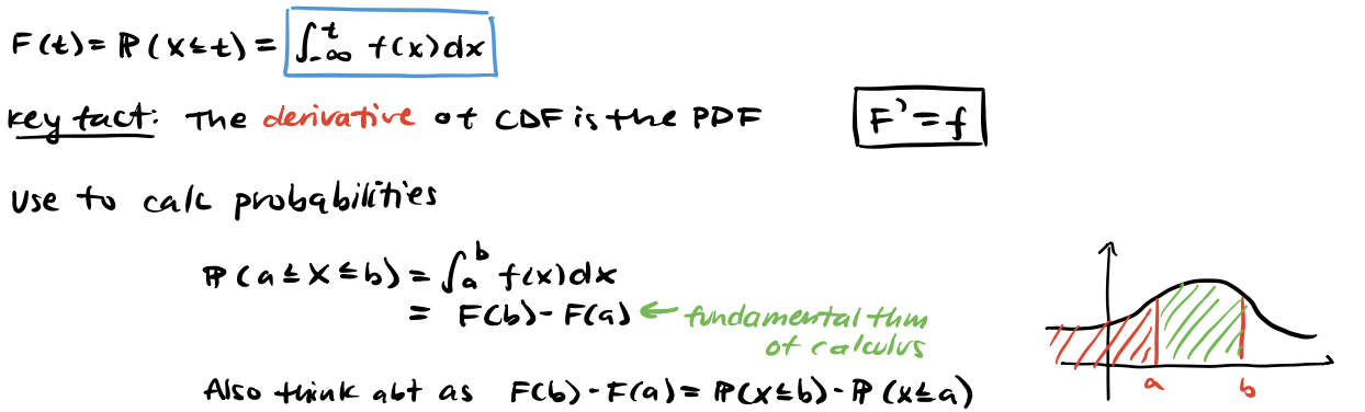
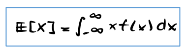
Expected Value of Continuous RV

Uniform: X~Unif[a,b]

E[X] = (a+b)/2

Var(X) = (b-a)²/12

Exponential: X~Exp(lambda)

Parameter: lambda > 0 (rate)

Models: Waiting times; (1) How long wait until next train (2) lambda = # arrivals per unit time on average

(vs. Poisson counts how many arrivals in one unit time)

E[X] = 1/(lambda)

Var(X) = 1/(lambda²)

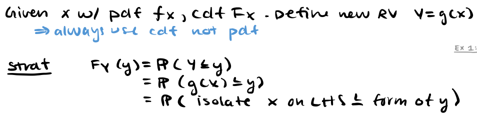
Transformations of RVs

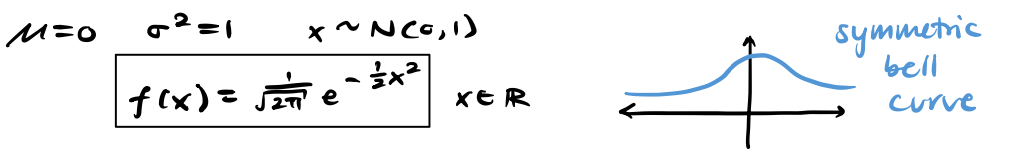
Normal Distribution: X~N(mu, sigma²)

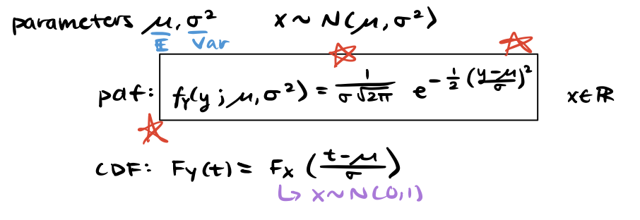
Standard Normal Distribution

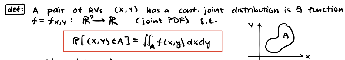
Continuous joint distributions

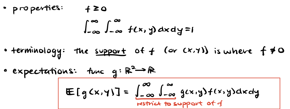
Continuous joint distributions properties & expected value

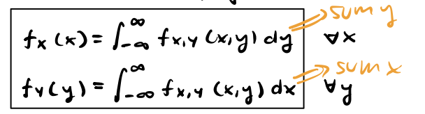
Marginal PDFs of Joint PDF

Independence of joint PDF (continuous)

Conditional PDF of X given Y

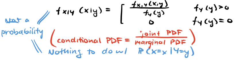
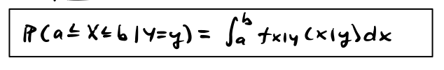
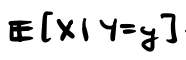
(Continuous)

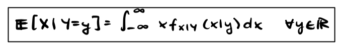
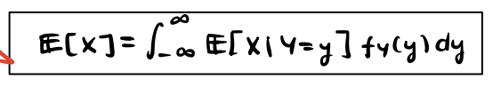
Law of total expectation with conditional PDF (continuous)

Tower Property (Law of Iterated Expectations)

Law of Total Variance (Conditional)

Consequence: Var(X) >= Var(E[X|Y]) always

Variance decreases after observing Y

X~Binomial(n,p):

E[X], E[X|Y=y], E[X|Y]

= np

= yp

= Yp

X~Binomial(n,p):

Var(Y), Var(X|Y=y), Var(X|Y)

= Var(Y)

= y*p*(1-p)

= Y*p*(1-p)

IID Random Vars (Independent & Identically Distributed)

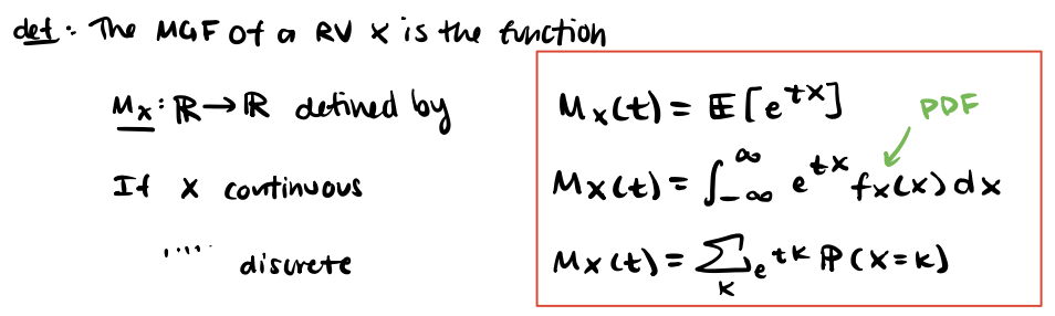
Moment Generating Functions (MGF)

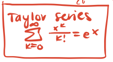
Taylor Series for e^x

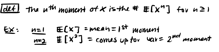
nth moment of X

(dMx/dt)(0), (d²Mx/dt²)(0), …, (dⁿMx/dtⁿ)(0)

E[X], E[X²], …, E[Xⁿ]

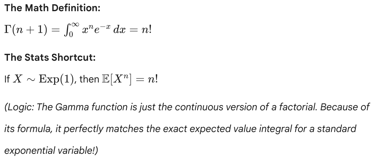
Gamma function: generalizes factorial to non-integer values

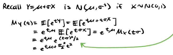
MGF of Normal Distribution N(mu, sigma²)

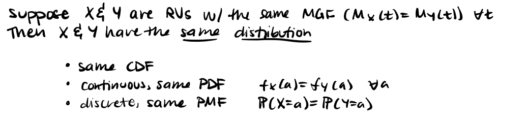
MGF: Inversion Theorem

Identify distributions from MGF form

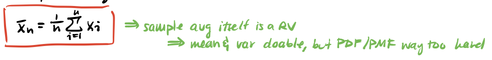
Sample Average of n of our RVs

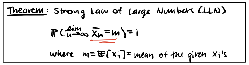
Strong Law of Large Numbers (LLN)

Weak Law of Large Numbers

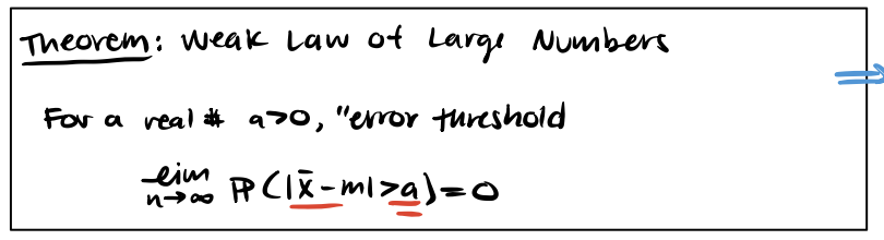
Error Probability

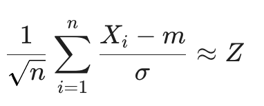
Central Limit Theorem (CLT)

Solve for m, sigma depending on the distribution. Plug into formula accordingly.

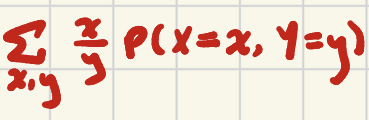
E[X/Y] - Discrete, Dependent

If independent, is it correlated?

If independent, it is uncorrelated BUT if uncorrelated, not necessarily independent.

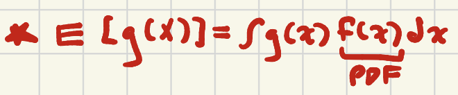
Continuous: E[g(X)]

Bounds: -inf, to inf

MGF of N(0,1)

M_x=e^t²/2

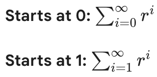
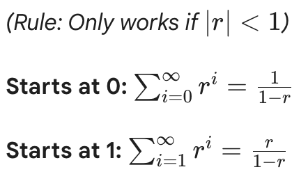
Infinite Geometric Series

Var(X+Y)

Var(X) + 2Cov(X,Y) + Var(Y)