Lecture 20: Business Cycle- AS/ AD Model application to Fiscal Policy

Fiscal policy

actions by the government (congress and the president) that change the levels of government spending & tax revenue. This change then affects aggregate demand.

Expansionary fiscal policy

• Government spending increases (due to things like defense spending and road construction), aggregate expenditure increases, and aggregate demand increases.

• Tax decreases, Disposable income increases, consumption increases, aggregate demand increases.

Recession graph + what two options does the government have

1) do nothing

2) Expansionary fiscal policy (stimulus)

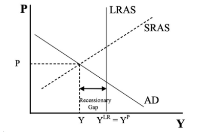
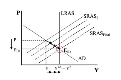
Option one analysis: do nothing

• Transition in the LR occurs automatically

• Due to the recessionary gap, there is less demand for labor, laborers have less bargaining power, labor costs/ input costs decrease, downward pressure on prices, SRAS will shift right in the LR, returning to Y^p

• The problem? In a recession, individuals are suffering, and no intervention means the economy will take a very long time to self-correct because firms are typically reluctant to lower wages (and would rather lay off workers) so the adjustment across AD is very slow.

• In this case, the price ends up lower in the LR equilibrium.

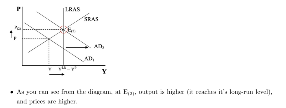
Option two analysis: Expansionary fiscal policy

• Bring output back up to its potential long-run level sooner!

• By increasing G or decreasing T, the government can make AD shift right, and bring the economy back to the potential level very quickly.

• Prices are higher in the long-run equilibrium

Difference between option 1 and 2

Although option one and two both achieve the same goal (returning to Y^LR ) they differ because…

1) Option 2 leads to Y^LR faster than option 1.

2) Option 2 increases price level, option 2 decreases price level.

The spending multiplier

• The amount by which overall output increases per unit increase in exogenous spending ( C, I, G, NX)

• FORMULA: ΔY= (1/ 1- MPC) ΔG ( or any exogenous change to AD)

Example: say the government increases spending by 50 in order to build roads. Desrcieb the direct effect and feedback effect. Asusme MPC is 0.8

• Direct Effect: Government spending increases, output increases, 50 units of gov spending = 50 units of road.

  • The production generates an equal amount of income in the economy. increase in output by 50 = increase of 50 in income

• Feedback Effect: When income goe sup by 50, some income will be saved and the rest consumed. Assume MPC is 0.8. Thus, consumption will increase by 0.8(50), which is 40.

  • The 40-unit increase in consumption, in turn, causes income to go up by 40. Again the MPC= 0.8 of the new income will be consumed which yield another round of the feedback effect.

• The total effect of 50 unit increase in gov spending woudl be: 50 (1/ (1-0.8))= 250

• This 250 represent by how much AD shifts out.

Relationship between spending multiplier and MPC

• The spending multiplier (in the case where consumption depends on income) is (1/ (1-MPC))

• The greater MPC, the greater the spending multiplier and the bigger shift of AD.

What does the spending multiplier not account for?

• In this model, we only assume one form of leakage (savings). In reality, there are many forms of leakage to consider like spending on imports.

• We also do not need account for investments. As income rises, investment would also rise, but this model does not account for that.

• We also assume MPC is the same for everyone- in actuality it varies.

Cost of using fiscal policy to stimulate the economy: Uncertainty about how much to spend and the danger of overshooting. (4 common issues with stimulus)

1) Inflation- Even when the magnitude of fiscal stimulus is just right, the boost in AD is accompanied by inflation. The more you overshoot the stimulus, the more inflation.

2) Predicting potential GDP- Economists also have a difficult time predicting the potential GDP level for an economy. Therefore, there is no clear-cut answer on how much stimulus an economy needs in a given period of time.

3) Spend v Save- With tax cuts,its also difficult to predict how much someone will spend versus save.

4) Timing- By the time a policy is passed, the economy may have already changed in the meantime.

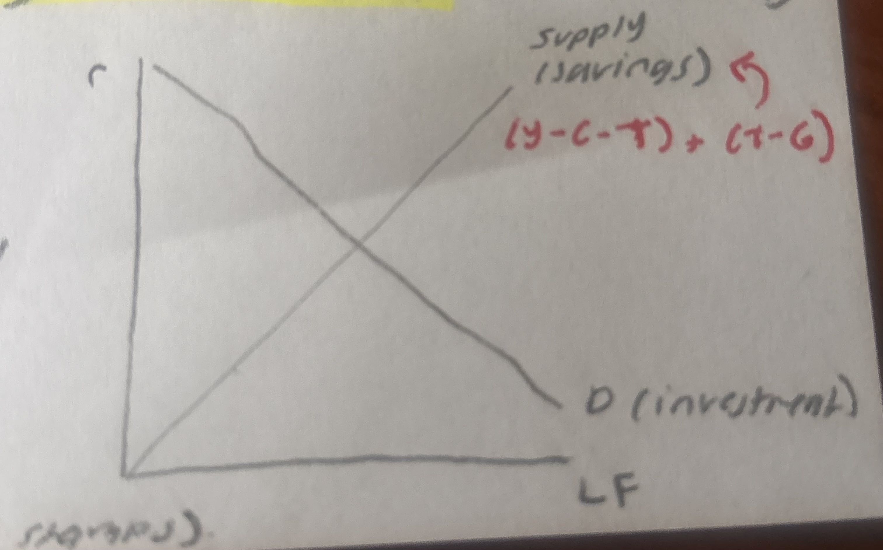
Loanable funds graph review

Cost of using fiscal policy to stimulate the economy: Crowding out- Short run

• When the government borrows in order to spend, interest rates tend to rise, crowding out private investment and consumption spending.

• Fiscal policy is much less effective in a more realistic economy where I and C depend on r as well as Y.

• crowding out is a factor that constrains AD.

Cost of using fiscal policy to stimulate the economy: Crowding out- long run

• Expansionary fiscal policy increases the government budget deficit, public savings decreases, in the loanable funds market this causes the quantity of loanable funds to decline, real intrest rate rises, reduction of investments and reduces growth of K.

• In AS/AD model this shifts LRAS left

• In All: expansionary fiscal policy leads to lower public savings, implies higher real interest rate rises, lower investment and capital, and therefore lower level of potential RGDP. This shifts LRAS to the left. Overtime expansionary fiscal policy can lead to higher prices and lower LR output levels

• Y₁^p < Y₂^p

What stronger alternatives exist?

• Measures known as automatic stabilizers. These include:

  • Income tax

  • Unemployment Benefits

  • Food Stamps