Block 1

Statistical Learning

Focuses on the foundations, model interpretation, and understanding how predictors relate to the outcome (Y). It provides long-lasting structural frameworks.Machine Learning / AI:

Machine Learning / AI

Prioritizes prediction accuracy, generalization, and handling highly complex, non-linear algorithms (like deep learning) where individual feature interpretation is often sacrificed ("black box" models)

Supervised Learning

You possess data containing both the predictors (X) and a known, observed outcome (Y). The model evaluates its performance directly against this known baseline

Unsupervised Learning

You only possess predictor data (X); there is no observed outcome variable Y. The goal shifts from prediction to discovering underlying groupings or patterns within the data. (CFA)

Training set

The portion of data used to build and fit your model.

Test set

A separate data split used to evaluate how well the model predicts on unseen observations. Evaluating performance only on your training data creates a severe risk of overfitting, as complex models will simply "memorize" data noise.

Internal Validation

Splitting a single, cohesive dataset into a training slice and a testing slice (e.g., a 70/30 split).

External Validation

Taking a model fully trained on one dataset (e.g., NHANES) and testing its predictive validity on an entirely separate population dataset collected elsewhere (e.g., Framingham).

Why does External datasets often fail? What are the methods?

Because they feature different parameter ranges, demographics, baseline mean values, or geographic variations. Methods to compensate for this include recalibration (adjusting model parameters or intercepts to match the new population's scale).

What is Data Leakage and what are solutions?

It is nformation from the test dataset that spills into the training workflow. For example, if you perform data imputation or scaling on the dataset before splitting it into train/test, your training step has seen the structure of the test data. We therefore impute and scale test data using only the "recipe" generated by the training data

What happens with interability when prediction accuracy increase?

As model complexity increases (e.g., moving from a simple linear fit to a flexible tree-based method like XGBoost), the model's accuracy improves. But the ability to interpret the variability impaact on the output drops.

The Bias-Variance Trade-off

Components: Error=Bias² +Variance + Irreducible Noise.

Principle that says that you cannot simultaneously minimize both sources of prediction error. As model complexity increases to reduce bias (better fitting), variance increases (higher sensitivity to training data). We want both for generalization.

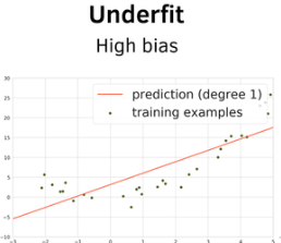
Bias (Underfitting)

False assumptions in your model type (e.g., fitting a perfectly straight line through data that actually follows a curved path). High-bias models miss major structural data patterns.

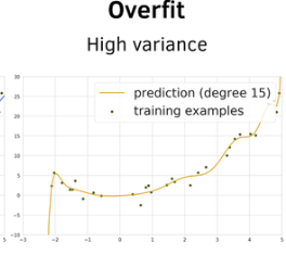
Variance (Overfitting)

Extreme model sensitivity to minor variations in your specific training dataset. High-variance models "connect the dots" perfectly, tailoring themselves to random data noise rather than the true signal.

Irreducible Noise

The fundamental variation in the environment or measurement tools that can never be filtered out, regardless of how flawless your model is.

The Parsimony Principle ("Less is More")

Models with fewer features are conceptually easier to interpret and less likely to suffer from high variance

Classical Selection Methods

All Subsets: A naïve strategy that tests every mathematical combination of your variables.

Forward Selection: Begins with an empty model, tests predictors one-by-one, extracts the single best variable, and iteratively adds variables until a specific stopping criterion (like a p-value threshold or a drop in Adjusted R²) is hit.

Backward Selection: Begins with all possible variables included in a single complex model, and iteratively strips away the variable providing the lowest statistical contribution to the fit.

Regularization / Penalization Concept

Way to stop model froom being too flexible (overfitting) adds a mathematical penalty to the objective function to constrain (shrink) the size of your regression coefficients (β) to be simpler and generalie better

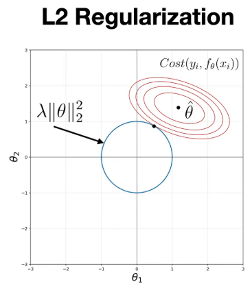
Ridge Regression (L2 Penalty)

Adds a penalty proportional to the size of the coefficients. It shrinks coefficients close to zero but never forces them to exactly zero; all variables remain inside the final model.

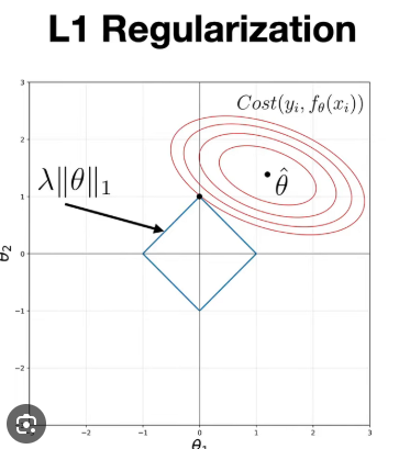
Lasso Regression (L1 Penalty):

Adds a penalty proportional to the absolute value of the coefficients. Because of its distinct geometric shape, Lasso forces less important coefficients to exactly zero, effectively acting as an automated variable selection tool.

The Scaling Mandate

Regularization methods are highly sensitive to data scales. If one variable is measured in thousands (e.g., blood cell counts) and another ranges from 0 to 1 (e.g., biological sex), the penalty term will unfairly squeeze the smaller-scaled variable. Therefore, features must be standard-scaled (mean = 0, SD = 1) before running Ridge or Lasso.

Non-Linear Concepts (Tree-based methods)

Algorithms that use a series of "if-then" rules to split complex, non-linear data into distinct, manageable regions. Unlike linear models, they require no data transformations.

Tree-Based Interactions

Unlike classical linear regressions which assume relationships follow standard straight lines, tree-based models (like XGBoost) naturally capture step-wise, non-linear boundaries and intricate multi-variable interactions without requiring you to manually write explicit interaction parameters (like age * BMI) into your formulas.

Handling Extreme Outliers (tree based method)

In linear regression, a severe outlier can radically skew your entire slope line. In tree-based models, outliers have a highly restricted impact because the model splits data based on internal value intervals (e.g., X > 150), meaning an extreme value of 1,000 behaves identically to a value of 151 during that split.

SHAPley (SHAP) Values (tree baseed method)

Method to measure how much each feature contributes to one specific prediciton. A SHAP value calculates how much a variable altered the final prediction for an individual person.

Missing Data & Imputation Theory

Values are unrecorded for variables of interest. Imputation theory provides statistical frameworks to estimate and replace these missing values, minimizing bias and preserving dataset size

The Feasibility of Imputation

Imputation is when a variable has a manageable amount of missingness (e.g., around 30%). However, if a variable is missing 50% or more of its data, or if the missingness is tied to an unobserved systemic bias, imputation becomes problematic and  bias.

Imputing Predictors vs. Outcomes

You should only use algorithms like K-Nearest Neighbors (K-NN) to impute missing independent predictors (X) by leveraging information from surrounding variables (e.g., using waist and hip measurements to impute a missing BMI value). You must never impute a missing target outcome variable (Y, such as sysBP). If the outcome is missing, that observation must be omitted from model training

The "Recipe" and Data Leakage Prevention

When performing validation, you split your data into training and test sets before imputation. You then create an imputation "recipe" based on the training data. This recipe is applied to the test data. If you mix the two datasets before imputing, you create data leakage.

Why External Validation Fails

Distribution and Range Discrepancies: External set that contains a wider range or completely different extreme values of systolic blood pressure (e.g., up to 295 mmHg vs. NHANES' 231 mmHg), the model is forced to extrapolate outside its learned boundaries.

Historical/Temporal Shifts: Baseline population statistics shift over generations due to public health interventions or cleaner living habits.

Compensating for Failure (Recalibration): If your model has solid predictive discrimination but systematically over- or under-predicts when applied to a new population, you can perform recalibration. This involves taking the frozen model and adjusting its parameters or updating the intercept (β₀) to align perfectly with the baseline risk metrics of the new geography or population.

Cross Sectional

Data collected from subjects at a single, fixed point in time. - Baseline demographic surveys

Longitudinal

The exact same subjects are tracked and measured repeatedly over a span of time - The Framingham Heart Study tracking cardiovascular health over decades