SOA Exam FM Master Review Flashcards

A comprehensive set of vocabulary flashcards covering interest theory, annuities, loans, bonds, duration, and immunization for the SOA Exam FM.

Effective Rate per Period (Nominal Rate Trick)

For a nominal rate $i^{(m)}$, the effective rate per period is expressed as $i^{(m)} / m$, not $i^{(m)}$.

Accumulation Function

Simple Interest

$</p><p>a(t)=1+it</p><p>$

Compound Interest

$</p><p>a(t)=(1+i)^t</p><p>$

Force of Interest

$</p><p>a(t)=e^{\delta t}</p><p>$

Discount Function

$</p><p>v(t)=\frac{1}{a(t)}</p><p>$

Accumulation Factor from Time \(s\) to Time \(t\)

$</p><p>\frac{a(t)}{a(s)}</p><p>$

Discount Factor from Time \(t\) to Time \(s\)

$</p><p>\frac{a(s)}{a(t)}</p><p>$

Interest Earned During Year \(n\)

$</p><p>I_n=a(n)-a(n-1)</p><p>$

Effective Interest Rate During Year \(n\)

$</p><p>i_n=\frac{a(n)-a(n-1)}{a(n-1)}</p><p>$

Effective Discount Rate During Year \(n\)

$</p><p>d_n=\frac{a(n)-a(n-1)}{a(n)}</p><p>$

Relationship Between Effective Interest and Effective Discount

$</p><p>d=\frac{i}{1+i}</p><p>$

$</p><p>i=\frac{d}{1-d}</p><p>$

\section*{Special Case: Simple Interest}

Accumulation Function

$</p><p>a(t)=1+it</p><p>$

Interest Earned During Any Year

$</p><p>I_n=i</p><p>$

Effective Interest Rate During Year \(n\)

$</p><p>i_n=\frac{i}{1+i(n-1)}</p><p>$

Effective Discount Rate During Year \(n\)

$</p><p>d_n=\frac{i}{1+in}</p><p>$

\section*{Special Case: Compound Interest}

Accumulation Function

$</p><p>a(t)=(1+i)^t</p><p>$

Interest Earned During Year \(n\)

$</p><p>I_n=i(1+i)^{n-1}</p><p>$

Effective Interest Rate During Every Year

$</p><p>i_n=i</p><p>$

Effective Discount Rate During Every Year

$</p><p>d_n=d=\frac{i}{1+i}</p><p>$

\section*{Force of Interest Relationships}

Accumulation Function

$</p><p>a(t)=e^{\delta t}</p><p>$

Discount Function

$</p><p>v(t)=e^{-\delta t}</p><p>$

Convert Force to Effective Interest

$</p><p>i=e^\delta-1</p><p>$

Convert Effective Interest to Force

$</p><p>\delta=\ln(1+i)</p><p>$

Accumulation Over \(t\) Years Using Force

$</p><p>(1+i)^t=e^{\delta t}</p><p>$

\section*{Useful FM Facts}

Present Value at Time 0 of Amount \(A\) at Time \(t\)

$</p><p>PV=A\,v(t)</p><p>$

Future Value at Time \(t\) of Amount \(A\) at Time 0

$</p><p>FV=A\,a(t)</p><p>$

Accumulation Function Must Satisfy

$</p><p>a(0)=1</p><p>$

For Compound Interest

$</p><p>a(t+s)=a(t)a(s)</p><p>$

For Simple Interest

$</p><p>a(t+s)\neq a(t)a(s)</p><p>$

Force of Interest Accumulation Factor

This is one of the highest-yield FM topics because it ties together accumulation functions, interest rates, discount rates, and calculus.

Here's the version I'd put in a cheat sheet.

---

Force of Interest ((\delta))What does Force of Interest represent?

The force of interest is the instantaneous rate of growth of an investment.

Think of it as:

"If I zoom in to an infinitely small moment in time, how fast is the account growing right now?"

For compound interest:

$$<br>\delta=\ln(1+i)<br>$$

For example, if

$$<br>i=8$$

then

$$<br>\delta=\ln(1.08)=0.07696<br>$$

Notice:

\delta<i

---

Definition of Force of Interest

Given an accumulation function (a(t)),

$$<br>\boxed{<br>\delta_t=\frac{a'(t)}{a(t)}<br>}<br>$$

Interpretation:

• Numerator = rate of change

• Denominator = current balance

So force of interest is:

$$<br>\frac{\text{growth per year}}{\text{current balance}}<br>$$

---

The Most Important Formula

Starting with

$$<br>\delta_t=\frac{a'(t)}{a(t)}<br>$$

we get

$$<br>a'(t)=\delta_t a(t)<br>$$

Integrating:

$$<br>\boxed{<br>a(t)=e^{\int_0^t \delta_s,ds}<br>}<br>$$

This is the master formula.

Whenever FM gives a force of interest, your first thought should be:

Integrate (\delta), then exponentiate.

---

Constant Force of Interest

If

$$<br>\delta_t=\delta<br>$$

is constant:

$$<br>a(t)=e^{\delta t}<br>$$

This is the continuous-compounding formula.

---

Relationship Between (i), (d), and (\delta)

Given force:

$$<br>i=e^\delta-1<br>$$

$$<br>d=1-e^{-\delta}<br>$$

Given effective interest:

$$<br>\delta=\ln(1+i)<br>$$

Given effective discount:

$$<br>\delta=-\ln(1-d)<br>$$

---

Quick Conversion Triangle

Starting with (i):

$$<br>d=\frac{i}{1+i}<br>$$

$$<br>\delta=\ln(1+i)<br>$$

Starting with (d):

$$<br>i=\frac{d}{1-d}<br>$$

$$<br>\delta=-\ln(1-d)<br>$$

Starting with (\delta):

$$<br>i=e^\delta-1<br>$$

$$<br>d=1-e^{-\delta}<br>$$

---

Discount Function

If

$$<br>a(t)=e^{\int_0^t \delta_s ds}<br>$$

then

$$<br>v(t)=\frac1{a(t)}<br>$$

Therefore

$$<br>\boxed{<br>v(t)=e^{-\int_0^t \delta_s ds}<br>}<br>$$

For constant force:

$$<br>v(t)=e^{-\delta t}<br>$$

---

Effective Interest Rate During Year (n)

If force varies with time:

$$<br>i_n=<br>\frac{a(n)-a(n-1)}<br>{a(n-1)}<br>$$

Using force:

$$<br>\boxed{<br>i_n=<br>e^{\int_{n-1}^{n}\delta_tdt}-1<br>}<br>$$

This shortcut appears often on FM.

---

Effective Discount Rate During Year (n)

$$<br>d_n=<br>\frac{a(n)-a(n-1)}<br>{a(n)}<br>$$

Using force:

$$<br>\boxed{<br>d_n=<br>1-e^{-\int_{n-1}^{n}\delta_tdt}<br>}<br>$$

---

Simple Interest and Force

Simple interest:

$$<br>a(t)=1+it<br>$$

Differentiate:

$$<br>a'(t)=i<br>$$

Thus

$$<br>\delta_t=<br>\frac{i}{1+it}<br>$$

---

Key Understanding

Simple interest does NOT have a constant force.

Instead:

$$<br>\boxed{<br>\delta_t=<br>\frac{i}{1+it}<br>}<br>$$

which decreases over time.

Example:

$$<br>i=8$$

At (t=0):

$$<br>\delta_0=0.08<br>$$

At (t=5):

$<br>\delta_5=<br>\frac{0.08}{1.4}</p><p>0.0571<br>$

Force gets smaller as time passes.

---

Compound Interest and Force

Compound interest:

$$<br>a(t)=(1+i)^t<br>$$

Differentiate:

$$<br>a'(t)=<br>(1+i)^t\ln(1+i)<br>$$

Thus

$$<br>\delta_t=<br>\ln(1+i)<br>$$

which is constant.

Therefore:

$$<br>\boxed{<br>\delta=\ln(1+i)<br>}<br>$$

---

Deriving (a(t)) from Force Quickly

When given (\delta_t):

Step 1

Integrate

$$<br>\int_0^t \delta_s ds<br>$$

Step 2

Exponentiate

$$<br>a(t)=e^{\int_0^t\delta_s ds}<br>$$

Step 3

Simplify

---

Example:

$$<br>\delta_t=\frac{2}{10+t}<br>$$

Integrate:

$<br>\int_0^t \frac{2}{10+s}ds</p><p>2\ln\left(\frac{10+t}{10}\right)<br>$

Exponentiate:

$<br>a(t)</p><p>e^{2\ln((10+t)/10)}<br>$

$$<br>\boxed{<br>a(t)=\left(\frac{10+t}{10}\right)^2<br>}<br>$$

---

FM Shortcut for Finding (a(t))

When you see

$$<br>\delta_t=<br>\frac{k}{a+bt}<br>$$

immediately think

$<br>\int \frac{k}{a+bt}dt</p><p>\frac{k}{b}\ln(a+bt)<br>$

and therefore

$<br>a(t)</p><p>\left(\frac{a+bt}{a}\right)^{k/b}<br>$

This pattern appears repeatedly on FM.

---

Three Facts to MemorizeConstant force

$$<br>a(t)=e^{\delta t}<br>$$

Simple interest

$$<br>\delta_t=\frac{i}{1+it}<br>$$

Compound interest

$$<br>\delta=\ln(1+i)<br>$$

If you know those three formulas plus

$$<br>a(t)=e^{\int_0^t\delta_s ds},<br>$$

you can solve essentially every FM force-of-interest problem.

Annuity-Immediate

Payments of $1$ at the end of each period for $n$ periods, with $PV = a_{n|} = (1 - v^n) / i$.

Annuity-Due

Payments at the beginning of each period, where $\ddot{a}_{n|} = (1 + i) a_{n|}$.

Deferred Annuity ($k|a_{n|}$)

An annuity valued at time $k$ and then discounted back $k$ periods using $v^k \cdot a_{n|}$.

Perpetuity

Immediate: An annuity with payments continuing forever, with a present value of $1/i$.

Due: An annuity with payments continuing forever starting at time $0$, with a present value of $1/d$.

Geometric: A perpetuity where payments grow by rate $g$ each period, valid if g < i, with a value of $1 / (i - g)$.

Increasing Arithmetic

Decreasing Arithmetic

Increasing Annuity-Immediate ($Ia_{n|}$)

An annuity with payments of $1, 2, 3, \dots, n$ ; valued as $Ia=(\ddot{a}_{n|}-nv^{n})/i$.

Decreasing Annuity-Immediate ($Da_{n|}$)

An annuity with payments of $n, n - 1, \dots, 1$; valued as $(n - a_{n|}) / i$.

Arithmetic Identity

$$(Ia)_{n|} + (Da)_{n|} = (n + 1) a_{n|}$$

Continuous Level Annuity

The present value (PV) of receiving $1 per year continuously for n years is defined as:

 $\overline{a}_{\overline{n}|} = \lim\_{m \to \infty} a\_{\overline{n}\|}^{(m)} = \frac{1 - v^{n}}{\delta}$  $= \frac{i}{\delta} \cdot \frac{1 - v^{n}}{i} = \frac{i}{\delta} a\_{\overline{n}\|}$.

The accumulated value (AV) for the same annuity is described as:

 $s\_{\overline{n}\|} = \overline{a}\_{\overline{n}\|}(1 + i)^{n}$  $= \frac{1}{\delta}(\overline{a}\_{\overline{n}\|}(1 + i)^{n}) = s\_{\overline{n}\|}$.

Varying Continuous Annuity

The present value (PV) of a continuous annuity with varying payment rate $f(t)$ and force of interest $\delta_t$ is defined as:

$PV = \int_0^n f(t) \exp\left(-\int_0^t \delta_s \,ds\right) dt.$

The accumulated value (AV) is given by:

$AV = \int_0^n f(t) \exp\left(\int_t^n \delta_s \,ds\right) dt.$

If $f(t) = t$ for a continuous increasing annuity:

$$(\overline{Ia})_{\overline{n}|} = \int_0^n t \, v^t \, dt = \frac{\overline{a}_{\overline{n}|} - n v^n}{\delta}.$$

$$(\overline{Is})_{\overline{n}|} = \int_0^n t (1+i)^{n-t} \, dt = (\overline{Ia})_{\overline{n}|} (1+i)^n.$$

$(\overline{Ia})_{\infty} = \frac{1}{\delta^2}.$

For a continuous decreasing annuity where $f(t) = n - t$:

$$(\overline{Da})_{\overline{n}|} = \int_0^n (n-t) v^t \, dt = \frac{n - \overline{a}_{\overline{n}|}}{\delta}.$$

$$(\overline{Ds}){\overline{n}|} = \int_0^n (n-t)(1+i)^{n-t} \, dt = (\overline{Da}){\overline{n}|} (1+i)^n$$

Prospective Outstanding Balance ($OB_k$)

The present value of remaining payments: $PMT \cdot a_{\overline{n-k}|}$.

Retrospective Outstanding Balance ($OB_k$)

The accumulated value of the loan minus the accumulated value of payments: $L(1 + i)^k - PMT \cdot s_{\overline{k}|}$.

Sinking Fund Method

A loan repayment method where the borrower pays interest to the lender and separately accumulates a fund at rate $j$ to repay the principal in one lump sum.

IRR (Internal Rate of Return)

The interest rate $r^*$ that sets the Net Present Value (NPV) of a cash flow stream to zero.

Dollar-Weighted Rate of Return (DWRR)

The rate of return equivalent to the IRR on a fund, which is affected by the timing and size of external cash flows.

Time-Weighted Rate of Return (TWRR)

A measure of a fund manager's performance that eliminates the effect of external cash flows by chain-linking sub-period returns.

Par Bond

A bond where the coupon rate $r$ equals the yield rate $i$, resulting in the Price $P$ equaling the Redemption Value $C$.

Premium Bond

A bond where the coupon rate $r$ is greater than the yield rate $i$ ($r > i$), resulting in a Price $P > C$.

Discount Bond

A bond where the coupon rate $r$ is less than the yield rate $i$ ($r < i$), resulting in a Price $P < C$.

Premium/Discount Formula

$$P = C + (Fr - Ci) a_{n|}$$

Makeham Formula

$P = K + \frac{g}{i} (C - K)$, where $K = C v^n$ and $g = Fr / C$.

Callable Bond Pricing

The process of pricing a bond at every possible call date and selecting the minimum price to account for the worst-case yield.

Spot Rate ($s_t$)

The effective annual rate for an investment made from time $0$ to time $t$.

Forward Rate ($f_{t,m}$)

The rate agreed upon today for lending that occurs from time $t$ to time $t + m$.

No-Arbitrage Relationship

$$(1 + s_{t+m})^{t+m} = (1 + s_t)^t \cdot (1 + f_{t,m})^m$$

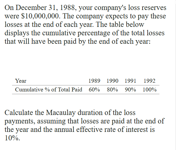
Macaulay Duration ($D\_{Mac}$)

Macaulay Duration (MacD) is a measure of the average time until cash flows from a financial asset are received, weighted by the present value of those cash flows. Mathematically, it is defined as:

$$MacD = \frac{\sum t A\_t}{P} = -\frac{\frac{d}{d\delta} P\_{\delta}}{P\_{\delta}}$$

where:

• $P$ = price of the asset

• $A\_t$ = present value of the cash flow at time $t$

---

Interpretation:

• MacD represents the average time at which cash flows occur, considering their present value.

• If there is only one cash flow, then:   $MacD = \text{time until that cash flow occurs}$

• A bond with higher coupon payments tends to have a shorter MacD.

• A bond with a higher yield also tends to have a shorter MacD.

---

Par Bond Shortcut: If a bond is priced at par, MacD can be approximated as:

$$MacD = \ddot{a}\_{\overline{n}\|}^{(m)} - \frac{1}{m} a\_{\overline{n}\|mj}$$

where:

• $j = \frac{i^{(m)}}{m}$ is the effective interest rate per period.

• $m$ = number of coupon payments per year.

---

Important Note:

• The par value of the bond does not influence MacD.

• If not specified, it is common to use a par value of 100.

---

Duration of a Portfolio: The MacD for a portfolio of multiple assets is defined as:

$$MacD\_P = \frac{P\_1 MacD\_1 + P\_2 MacD\_2 + \cdots + P\_n MacD\_n}{P\_1 + P\_2 + \cdots + P\_n}$$

where:

• $P\_i$ = market price of asset $i$

• $MacD\_i$ = MacD of asset $i$

---

Approximation Using Macaulay Duration: The future price of a bond can be approximated as:

$$P\_{i\_1} \approx P\_{i\_0} \left( \frac{1+n\_0}{1+n\_1} \right)^{MacD}$$

where:

• $P\_{i\_0}$ = price at the original effective annual yield $i\_0$

• $P\_{i\_1}$ = price at the new effective annual yield $i\_1$

---

Notes:

• It is crucial to express interest rates as effective annual rates since MacD is measured in years.

• Using MacD provides a better price approximation compared to Modified Duration when cash flows are positive.

---

FM Memory Box: Macaulay Duration = weighted average time of cash flows

To remember this concept, think of: $MacD = \frac{\text{Time-Weighted PV of Cash Flows}}{\text{Price}}$

Quick Facts:

• Higher coupon rate ⟹ Lower Duration

• Higher yield ⟹ Lower Duration

• Zero-coupon bond ⟹ MacD = maturity

• Portfolio duration = weighted average of component durations

• The par bond shortcut is a key concept in financial mathematics

• MacD is measured in years

Modified Duration ($D\\_{Mod}$)

Modified Duration (ModD) quantifies a bond's price sensitivity to changes in yield. It is mathematically defined by:

$$ModD = -\frac{1}{P} \frac{dP}{di}$$

where:

• $P$ = price of the bond,

• $dP$ = change in price due to yield change,

• $di$ = change in yield.

Interpretation: This formula allows us to approximate the percentage change in price for small changes in yield:

$$\frac{\Delta P}{P} \approx -ModD \cdot \Delta i$$

• A larger ModD indicates greater sensitivity to interest rate fluctuations.

• ModD serves as the slope of the price-yield curve, illustrating the inverse relationship between interest rates and bond prices.

---

Relationship Between Modified Duration and Macaulay Duration:

The relationship can be expressed as:

$$ModD = v \cdot MacD = \frac{MacD}{1+i}$$

where:

• $v = \frac{1}{1+i}$ is the present value factor.

Equivalently, Macaulay Duration (MacD) can be expressed as:

$$MacD = (1+i)ModD$$

---

Macaulay Duration (MacD):

Macaulay Duration is defined as:

$$MacD = \frac{\sum t A\\_t}{P} = -\frac{\frac{d}{d\delta} P\\_{\delta}}{P\\_{\delta}}$$

Interpretation:

• MacD represents the weighted average time until cash flows are received, measured in years.

• For a single cash flow, it simplifies to:

$$MacD = \text{time until that cash flow occurs}$$

• For zero-coupon bonds:

$$MacD = \text{maturity}$$

Higher coupon bonds generally exhibit shorter MacD values, as do bonds with higher yields.

---

Approximating Bond Prices Using MacD:

To approximate bond prices when yields are expressed as effective annual rates:

$$P\\_{i\\_1} \approx P\\_{i\\_0} \left( \frac{1+i\\_0}{1+i\\_1} \right)^{MacD}$$

where:

• $P\\_{i\\_0}$ = price at yield $i\\_0$

• $P\\_{i\\_1}$ = price at yield $i\\_1$.

---

When to Use ModD:

Utilize ModD when you need:

• An approximate percentage change in price due to small yield changes,

• To assess the sensitivity of the bond price to interest rate changes,

• An answer to questions regarding price sensitivity:

$\frac{\Delta P}{P}$ or "How sensitive is price to yield?"

---

When to Use MacD:

Opt for MacD when:

• You are analyzing the average timing of cash flows,

• Engaging in duration matching or immunization strategies,

• Approximating bond prices with:

$P\\_{i\\_1} \approx P\\_{i\\_0} \left( \frac{1+i\\_0}{1+i\\_1} \right)^{MacD}$,

• Considering interest rates expressed as effective annual yields.

---

FM Memory Box:

• $$MacD = \text{Weighted Average Time}$$

• $$ Mod

Convexity ($C$)

A measure of the curvature of the price-yield curve, calculated as $C = \frac{1}{P} \frac{d^2P}{dt^2} = \frac{1}{P} \sum \frac{t(t + \frac{1}{m})v^{t + 2} \cdot CF_{t}}{(1 + i)^{t}} = \frac{1}{P} \sum \frac{t(t + \frac{1}{m})v^2 \cdot PV\left(CF_{t}\right)}{(1 + i)^{t}}$.

Convexity ($C$) measures the sensitivity of the duration of a bond to changes in interest rate, indicating how the price of a bond changes as interest rates fluctuate (second derivative of Price formula).

Where:

• $C$ = Convexity
  

• $P$ = Price of the bond
  

• $t$ = Time period
  

• $CF_{t}$ = Cash flow at time $t$
  

• $i$ = Yield to maturity
  

• $v$ = Present value factor, calculated as $v = \frac{1}{1 + i}$.

Redington Immunization

A strategy to protect against small parallel yield shifts by matching PV of assets and liabilities, matching durations, and ensuring Asset Convexity > Liability Convexity.

Full Immunization

A strategy that protects against any single yield shift by requiring asset cash flows to bracket liability cash flows (one before, one after).

Portfolio Yield Method

A method where new investments earn the same rate as the existing portfolio average.

New Money Method

Also known as the investment year method; new investments earn a rate based on current market conditions, tracked separately by cohort.

Zero-Coupon Bond Cheat Sheet

Definition: A zero-coupon bond pays:

• ✅ No coupons

• ✅ One payment at maturity
  

Key Formulas:

1. Price: $P = C v^n$

2. Duration: $D = n$

3. Yield: $i = \frac{C}{P}^{1/n} - 1$

4. Book Value: $BV_t = C v^{-(n-t)}$
   

Properties:

• Highest duration for a given maturity.

• Most price sensitive to interest rate changes.

• No reinvestment risk.

• Highest convexity.

• Ideal for immunization strategies.
  

FM Exam Clues: Remember these facts for zero-coupon bonds:

• One payment only

• Duration = Maturity

• Highest duration

• Highest interest-rate sensitivity.

Interest Rate Behavior

Connection with Bond Prices:

• When interest rates fall, bond prices increase.

• Long-term bonds are more sensitive to interest rate changes than short-term bonds because they have a higher duration.

• Low-interest-rate bonds benefit more in percentage terms when rates drop.

• In a falling rate environment, the bond that offers the most price sensitivity maximizes profit opportunity.

Common Linh’s mistake

Duration:

• First payment at time 0 as will be multiplied by 0!

• whenever you see a cumulative loss payment pattern, immediately convert it to incremental payments by taking differences between consecutive cumulative percentage

Special Case: Simple Interest

Accumulation Function: $a(t)=1+it$. The interest earned during any year is given by $I_n=i$ and the effective interest rate during year $n$ is $i_n=\frac{i}{1+i(n-1)}$. Effective discount rate during year $n$ is $d_n=\frac{i}{1+in}$.

Special Case: Compound Interest

Accumulation Function: $a(t)=(1+i)^t$. The interest earned during year $n$ is given by $I_n=i(1+i)^{n-1}$, and the effective interest rate during every year is $i_n=i$. The effective discount rate during every year is $d_n=d=\frac{i}{1+i}$.