Cell Biology Exam 3
1/140
There's no tags or description
Looks like no tags are added yet.
Name | Mastery | Learn | Test | Matching | Spaced | Call with Kai | Chat |
|---|
No analytics yet
Send a link to your students to track their progress
141 Terms
Why Nuclear Transport Matters
Why Nuclear Transport Matters
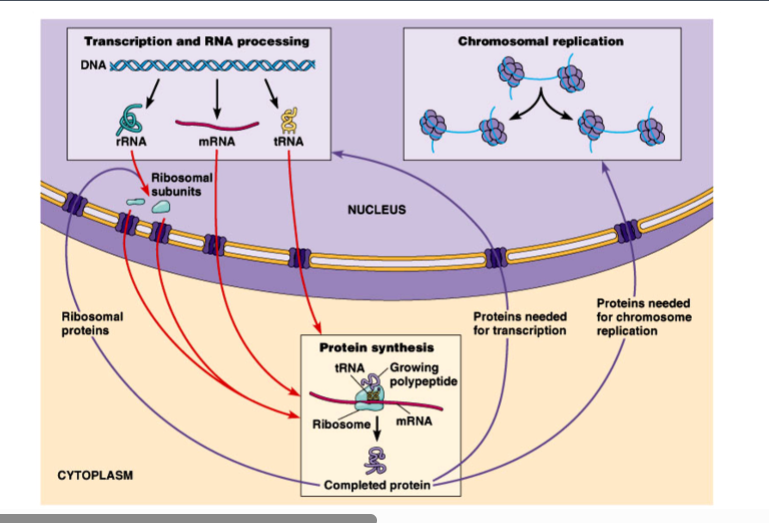
The nucleus requires a massive, continuous exchange of molecules with the cytoplasm to sustain normal cell function. The scale of this transport is enormous:
• A rapidly dividing HeLa cell (a common cancer cell line) must generate roughly 14,000 ribosomal subunits per minute and export them into the cytoplasm.
• Simultaneously, approximately 550,000 ribosomal proteins must be imported into the nucleus every minute to support ribosome assembly.
• Beyond ribosomal proteins, all proteins required for DNA replication and transcription must also be imported into the nucleus.
• Each individual nuclear pore handles about 4-5 ribosomal subunit passages per minute, meaning a ribosomal subunit passes through roughly every 10-12 seconds per pore — yet thousands of pores work in parallel to meet demand.
Morphology and Structure of the Nucleus
2.1 Basic Compartments
• The interior of the nucleus is called the nucleoplasm, which contains chromatin (decondensed chromosomes in non-dividing cells).
• The dark-staining central region visible in electron micrographs is the nucleolus — discussed in detail later.
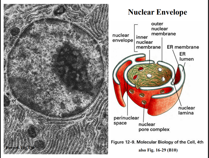
2.2 The Nuclear Envelope
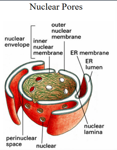
• The nucleus is surrounded by the nuclear envelope, a double membrane structure consisting of an inner nuclear membrane and an outer nuclear membrane.
• The space between the two membranes is the perinuclear space, which is continuous with the lumen of the endoplasmic reticulum (ER).
• The nuclear envelope is therefore best thought of as a specialized projection of the ER — this is why the rough ER is always found adjacent to the nucleus in micrographs.
• Ribosomes can be seen on the outer nuclear membrane, co-translationally inserting newly made polypeptides into the perinuclear space, exactly as they do on the rough ER.
• The inner nuclear membrane is supported on its nucleoplasmic face by a meshwork of protein fibers called the nuclear lamina, which provides structural support to the envelope.
2.3 Nuclear Pores
• Visible in the nuclear envelope are constriction points about 60-70 nm in width — these are the nuclear pores.
• In a thin-section EM image you might see ~10 pores, but the full 3D nucleus contains not hundreds but thousands of nuclear pores.
• Deep-etch freeze-fracture micrographs reveal the nuclear surface is covered in divot-like craters, each corresponding to a nuclear pore — the gateways for all nuclear transport.
• Many micrographs show a zone of exclusion immediately surrounding each pore on the nuclear side — the reason for this is still under active investigation.
The Nuclear Pore Complex (NPC)
3.1 Size and Composition
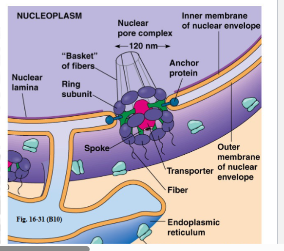
• Each nuclear pore is filled by the nuclear pore complex (NPC), a macromolecular assembly of ~120 megadaltons in total mass.
• The NPC is approximately 30 times the size of a ribosome — making it one of the largest protein complexes in the cell.
• It is composed of at least 30 different types of polypeptides (nucleoporins).
• Many of the nucleoporins lining the central channel are intrinsically disordered proteins — they lack a fixed 3D structure and move about like spaghetti. This disordered nature is critical to the NPC's selective barrier function.
3.2 Architecture — Octagonal Symmetry
• The NPC has 8-fold (octagonal) symmetry.
• On the cytoplasmic face: 8 protein subunits arranged in a ring around a central passageway.
• On the nucleoplasmic face: the same 8-fold symmetry, but the structure is more elaborate — it forms a basket or fish-net structure that protrudes into the nucleoplasm.
• In the center of these 8 passageways sits a 9th central transporter — this is the main channel for larger cargo molecules.
Two Modes of Transport Through the NPC
Two Modes of Transport Through the NPC
• Non-selective passive transport: molecules smaller than 40 kDa or less than 10 nm in diameter can diffuse freely through any part of the NPC, driven purely by concentration gradients. Ions move this way.
• Selective indirect active transport: molecules larger than 40 kDa or 10-30 nm in diameter require a specific transport machinery (see Section 4). Free energy is used — indirectly, via a concentration gradient ultimately maintained by GTP hydrolysis. Molecules larger than ~30 nm cannot enter the nucleus at all.
Experimental Evidence for the Size Limit — Gold Particle Experiments
Experimental Evidence for the Size Limit — Gold Particle Experiments
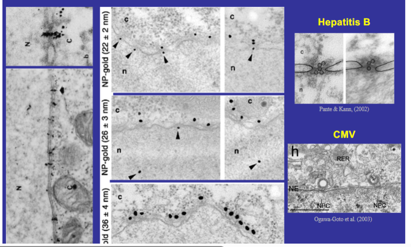
Elegant experiments using gold particles of defined diameter coated with nuclear-targeted proteins established the upper size limit for nuclear import:
• Gold particles 22 nm in diameter: found on both sides of the nuclear envelope — confirming entry into the nucleus.
• Gold particles 26 nm: same result — still able to enter.
• Gold particles 36 nm: accumulated at the nuclear envelope but could not enter the nucleoplasm — the boundary is ~30 nm.
• The gold particles entering the nucleus were always found concentrated at discrete regions of the nuclear envelope, corresponding to nuclear pore complexes — proving the NPC is the sole entry point.
• Real-life relevance: Hepatitis B virions (small enough) enter the nucleus through nuclear pore complexes. CMV (cytomegalovirus), too large to fit through, instead binds atop the NPC ring and injects its nucleic acid directly into the nucleus, leaving the capsid behind.
The Molecular Machinery of Nuclear Import
Three Essential Components
Three molecular components are required for selective nuclear import:
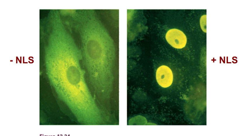
(1) Nuclear Localization Signal (NLS)
• A stretch of amino acids (roughly 20-30 residues) within the cargo protein that marks it for nuclear import.
• The NLS does not have a single strict consensus sequence — its exact sequence varies — but it is consistently enriched in basic residues: lysine and arginine.
• Experimental proof: attaching an NLS to a protein causes it to accumulate inside the nucleus. Removing the NLS from a nuclear protein causes it to remain in the cytoplasm.
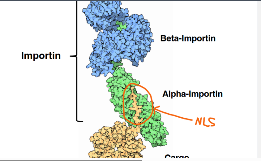
(2) Importin (the NLS receptor)
• Importin is a heterodimeric protein composed of alpha and beta subunits.
◦ Alpha-importin directly binds the NLS of the cargo protein.
◦ Beta-importin interacts with the nuclear pore complex, enabling translocation.
• Together, alpha + beta importin constitute the full importin complex.
• The cargo protein (carrying its NLS) bound to importin is the transport-competent cargo complex.
(3) RAN GTPase
• RAN is a small monomeric GTPase — the third family of small GTPases encountered in the course (after ARF and Rab families).
• Like all small GTPases: GDP-bound = OFF state; GTP-bound = ON state.
• Two key regulators:
◦ GEF (Guanine Nucleotide Exchange Factor): replaces GDP with GTP, activating RAN. The RAN-GEF is tethered to chromatin and is therefore exclusively nuclear.
◦ GAP (GTPase Activating Protein): stimulates GTP hydrolysis, inactivating RAN. The RAN-GAP has no NLS and is therefore exclusively cytoplasmic.
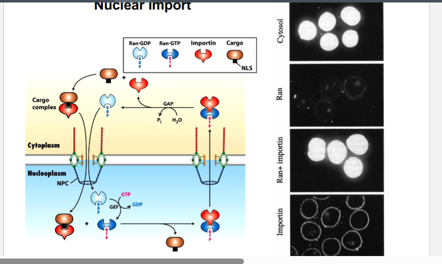
Step-by-Step Mechanism of Nuclear Import
Step-by-Step Mechanism of Nuclear Import
• Step 1 (Cytoplasm): The cargo protein (with its NLS) binds alpha-importin. Beta-importin associates to form the full cargo-importin complex.
• Step 2 (NPC): The cargo-importin complex moves through the central transporter of the nuclear pore complex from cytoplasm into nucleoplasm.
• Step 3 (Nucleus): Inside the nucleus, RAN-GTP (generated by the chromatin-associated GEF) binds to the importin complex, causing a conformational change that releases the cargo. The cargo is now free in the nucleus.
• Step 4 (Recycling): RAN-GTP + importin (without cargo) is exported back through the NPC into the cytoplasm.
• Step 5 (Regeneration): In the cytoplasm, RAN-GAP stimulates GTP hydrolysis, converting RAN-GTP to RAN-GDP. RAN-GDP dissociates from importin. Importin is free for another round of import. RAN-GDP re-enters the nucleus where GEF reactivates it to RAN-GTP.
In Vitro Reconstitution — How This Was Worked Out
In Vitro Reconstitution — How This Was Worked Out
The requirements for nuclear import were determined by reconstituting the process in a test tube (Gorlich et al., 1994):
• BSA (bovine serum albumin) was conjugated to fluorescein (a fluorescent dye) AND an NLS, then mixed with isolated nuclei and various cytosolic fractions.
• Nuclei + cytosol + NLS-BSA: BSA entered the nucleus (positive control).
• Nuclei + RAN alone: no fluorescence inside nuclei — RAN alone is insufficient.
• Nuclei + importin alone: fluorescence appeared around the nucleus (importin can deliver cargo to the nuclear envelope) but BSA did not enter — importin alone is insufficient.
• Nuclei + RAN + importin + NLS-BSA: BSA successfully entered the nucleus — demonstrating that all three components are necessary.
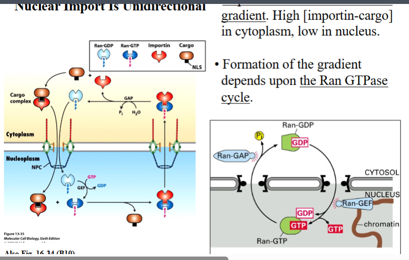
Why Nuclear Import Is Unidirectional
Why Nuclear Import Is Unidirectional
Nuclear import does not simply move cargo randomly in both directions — it is a directed, one-way process. Two mechanisms enforce directionality:
5.1 Concentration Gradient of the Cargo Complex
• The cargo-importin complex exists at HIGH concentration in the cytoplasm (where cargo is synthesized) and LOW concentration in the nucleus.
• Transport is therefore DOWN a concentration gradient — thermodynamically favorable.
• Although cargo is deposited in the nucleus, it immediately dissociates from importin (due to RAN-GTP), so the cargo-importin complex is never able to build up in the nucleus. The concentration of the cargo-importin complex remains low in the nucleus.
5.2 The RAN-GTP Gradient
• RAN-GTP concentration is HIGH in the nucleus and LOW in the cytoplasm — this asymmetry is what drives directionality.
• This gradient is maintained by the strict compartmentalization of the two RAN regulators:
◦ RAN-GEF is anchored to chromatin, so it is exclusively nuclear. GTP loading of RAN only occurs inside the nucleus.
◦ RAN-GAP is cytoplasmic (it has no NLS), so GTP hydrolysis only occurs in the cytoplasm.
• Consequence: GTP-RAN accumulates in the nucleus and triggers cargo release there; GDP-RAN accumulates in the cytoplasm, allowing importin to pick up new cargo there. The system cannot run in reverse.
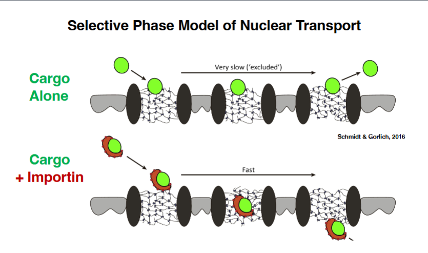
How Importin Enables Passage Through the NPC — The Selective Phase Model
How Importin Enables Passage Through the NPC — The Selective Phase Model
• The central channel of the NPC is lined by FG-nucleoporins — nucleoporins enriched in FG (phenylalanine-glycine) repeats.
• These FG-nucleoporins are intrinsically disordered proteins; they interact with each other and form a hydrogel — a dense, gel-like meshwork inside the central transporter.
• This hydrogel acts as a diffusion barrier: a cargo protein approaching the NPC without an escort cannot disrupt the FG-FG interactions and is effectively excluded. Entry would be so slow it is functionally impossible.
• However, when cargo is bound to importin, the surface of importin makes specific contacts with the FG-nucleoporins. These contacts disrupt the local FG-FG interactions, allowing the cargo-importin complex to penetrate the hydrogel rapidly and pass through.
• This mechanism — the hydrogel as barrier, importin as a 'hydrogel disruptor' — is called the Selective Phase Model of nuclear transport.
• Other models exist, but the selective phase model is currently the most widely supported.
• This explains why importin is essential even beyond simply recognizing the NLS: it physically enables passage through the NPC barrier.
The Nucleolus and Ribosome Biogenesis
The Nucleolus and Ribosome Biogenesis
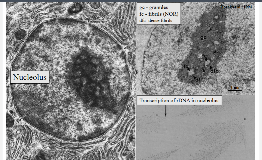
7.1 What Is the Nucleolus?
• The nucleolus is a distinct region within the nucleus, visible as a dark-staining area in EM and appearing like a droplet of oil inside the nucleus under a light microscope.
• It is not bounded by a membrane — it is maintained by phase separation (liquid-liquid demixing), and is now considered a biomolecular condensate.
• The phase separation means nucleolar contents are not freely mixing with the surrounding nucleoplasm — it maintains its own distinct biochemical environment.
Function of the Nucleolus — rRNA Synthesis and Ribosome Assembly
Function of the Nucleolus — rRNA Synthesis and Ribosome Assembly
• The nucleolus is the site of ribosomal DNA (rDNA) transcription, producing ribosomal RNA (rRNA) — the structural RNA component of ribosomes.
• Ribosomes = rRNA + ribosomal proteins. The rRNA is made here; the ribosomal proteins are synthesized in the cytoplasm, imported into the nucleus, and then imported into the nucleolus.
• As rRNA is being transcribed, ribosomal proteins immediately associate with it, assembling ribosomal subunits co-transcriptionally — visible in Oscar Miller's famous 1969 electron micrographs (performed in the basement of Gilmer Hall, UVA) as a 'Christmas tree' or feather-like pattern: the rDNA backbone with rRNA transcripts projecting perpendicularly, each tipped with ribosomal proteins.
• Once assembled, the ribosomal subunits must be exported from the nucleus into the cytoplasm where they will function.
Nucleolar Sub-Regions
• The rDNA is found in the lighter-staining fibrillar center (FC), also called the nuclear organizing region (NOR).
• The dense fibrillar component (DFC) is where active rDNA transcription and initial ribosomal subunit assembly occur.
• Completed or partially assembled subunits accumulate in the granular component (GC) before export
Nuclear Export
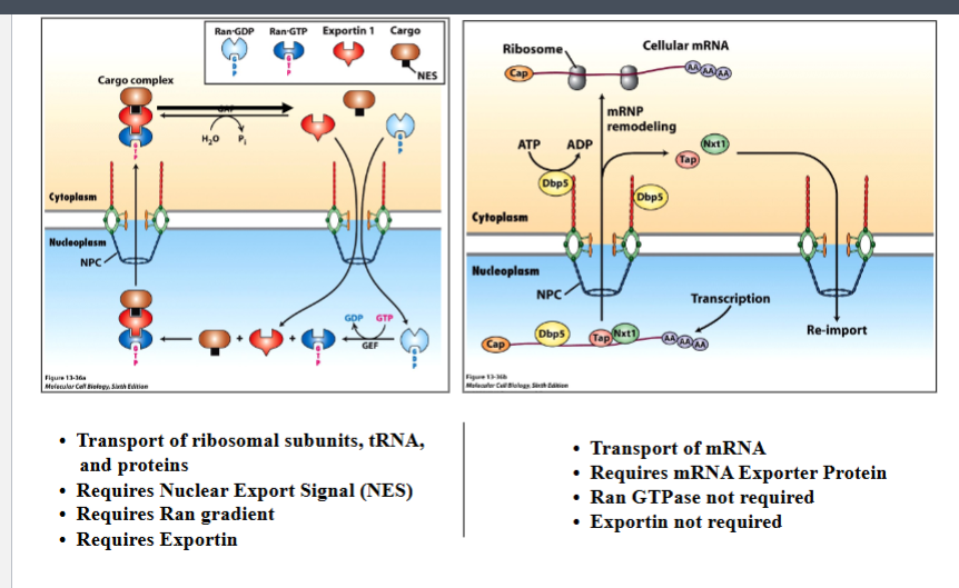
8.1 Export of Ribosomal Subunits, tRNA, and Proteins
Export of large molecules (ribosomal subunits, tRNA, and proteins bearing nuclear export signals) closely mirrors the import machinery:
• Requires a Nuclear Export Signal (NES) on the cargo — analogous to the NLS used for import.
• Requires RAN GTPase (the same RAN gradient drives export, just in the opposite direction relative to cargo movement).
• Requires Exportin — the export-dedicated receptor analogous to importin.
• Mechanistically: in the nucleus, RAN-GTP loads cargo onto exportin; the cargo-exportin-RAN-GTP complex exits through the NPC; in the cytoplasm, RAN-GAP converts RAN-GTP to RAN-GDP, causing cargo release and complex disassembly.
Export of mRNA — A Distinct Mechanism
• mRNA export uses a fundamentally different mechanism from the RAN/exportin pathway:
• Requires an mRNA exporter protein (e.g., Tap/Nxt1 complex in metazoans, associated with the mRNA as a messenger ribonucleoprotein, mRNP).
• Does NOT require the RAN GTPase gradient.
• Does NOT require exportin.
• The driving force for mRNA export involves ATP hydrolysis (by the Dbp5 helicase at the cytoplasmic face of the NPC) and mRNP remodeling, not the RAN cycle.
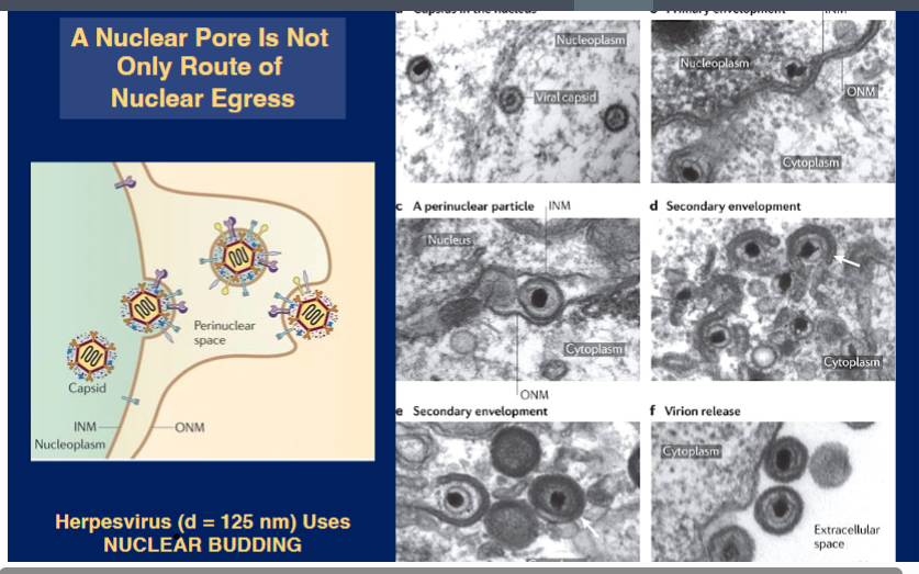
Nuclear Egress of Large Viruses — Nuclear Budding
Nuclear Egress of Large Viruses — Nuclear Budding
• A nuclear pore is not the only way to exit the nucleus — some viruses are too large even to consider using the NPC.
• Herpesvirus (diameter ~125 nm) uses a process called nuclear budding:
◦ Viral capsids assemble in the nucleoplasm.
◦ The capsid buds through the inner nuclear membrane, acquiring a temporary primary envelope and entering the perinuclear space.
◦ The primary envelope then fuses with the outer nuclear membrane, releasing the capsid into the cytoplasm.
◦ Secondary envelopment occurs in the cytoplasm, and mature virions are eventually released from the cell.
Review: Nuclear Import
Review: Nuclear Import
The lecture opened with a brief recap of nuclear import from the previous session. The key concepts are:
• Molecules larger than ~40 kDa (or >10 nm) cannot passively diffuse into the nucleus — they require active, selective transport through the Nuclear Pore Complex (NPC).
• The NPC has octagonal symmetry with a central transporter region rich in FG (phenylalanine-glycine) nucleoporins. These intrinsically disordered proteins form a hydrogel that acts as a selective barrier.
• Cargo cannot penetrate the hydrogel alone. When cargo binds importin (a carrier protein), the complex disrupts the hydrogel and moves through the pore — this is the Selective Phase Model of nuclear transport.
• Once inside the nucleus, Ran-GTP (bound to the GTPase Ran) breaks apart the importin-cargo complex. Cargo is released in the nucleoplasm; importin and Ran-GTP exit and are recycled.
• The entire process is driven by the Ran GTPase gradient: Ran-GTP is concentrated inside the nucleus (due to nuclear Ran-GEF associated with chromatin), while Ran-GDP predominates in the cytosol (Ran-GAP is cytoplasmic). This asymmetry makes import unidirectional.
Nuclear Export
Nuclear Export
Export from the nucleus also occurs through the NPC and mirrors the logic of import, but with important differences.
2a. General Export Mechanism (Ribosomal Subunits, tRNA, Proteins)
• Cargo that needs to leave the nucleus carries a Nuclear Export Signal (NES) — a short amino acid sequence (analogous to the NLS for import). NES sequences show considerable variation yet perform the same function.
• The NES is recognized by Exportin (the export counterpart of importin). Exportin, Ran-GTP, and the cargo form a ternary complex that moves through the NPC from the nucleoplasm to the cytoplasm.
• Once in the cytoplasm, GTP hydrolysis by Ran (assisted by Ran-GAP) disassembles the complex. Cargo stays in the cytoplasm; Exportin and Ran-GDP re-enter the nucleus for another round.
• Molecules that leave this way include: ribosomal subunits, tRNAs, and various proteins.
2b. mRNA Export — A Different Mechanism
• mRNA uses a distinct export pathway because it is translated in the cytoplasm and must leave in large quantities.
• mRNA is coated with a variety of proteins and exits via the mRNA Exporter Protein complex. Key point: Ran-GTPase and Exportin are NOT required for mRNA export — this is a distinct variation on the theme.
• The professor specifically advised against memorizing the names of all the individual proteins involved in mRNA export, as this detail is beyond the scope of the exam.
Comparison: Two Export Mechanisms
Feature | Standard Export (tRNA, ribosomes, proteins) | mRNA Export |
Carrier protein | Exportin | mRNA Exporter Protein |
Signal on cargo | Nuclear Export Signal (NES) | Protein coat on mRNA |
Ran-GTP required? | Yes | No |
Exportin required? | Yes | No |
Route | Nuclear Pore Complex | Nuclear Pore Complex |
Nuclear Budding — An Alternative Exit Route
Nuclear Budding — An Alternative Exit Route
The NPC is not the only way to exit the nucleus. Large complexes or viral particles that are too big to pass through the NPC can use a completely different mechanism.
• Example: Herpesvirus (diameter ~125 nm) — far too large for the NPC (central channel ~30 nm dilated).
Step-by-Step: Nuclear Budding Process
• The viral particle (nucleic acid + capsid) inside the nucleus interacts with the inner nuclear membrane (INM).
• The INM wraps around the viral particle, forming a membrane-coated virion. This enveloped particle is now located in the perinuclear space (the space between the inner and outer nuclear membranes).
• The membrane-coated virion then interacts with the outer nuclear membrane (ONM). Membrane fusion occurs, the membrane stays behind, and the viral particle is released into the cytoplasm.
• The virus then continues to the extracellular space via the normal secretory pathway.
• This entire process is called Nuclear Budding and is an active area of research — scientists are still working out the exact molecular machinery involved.
Why the Nucleus Has Been Difficult to Study
A. Historical Bias Toward the Cytoplasm
• Cell biology has historically focused on the cytoplasm, with the nucleus receiving comparatively little attention in both courses and the scientific literature.
• The American Society for Cell Biology (ASCB), founded in the 1960s, has been jokingly called the "American Society for Cytoplasm Biology" because the nucleus is rarely discussed at scientific meetings.
• Recent technological innovations have begun to reveal the complexity of the nucleus, making it less of an unknown territory (terra incognita).
B. Physical Challenges
• Cell fractionation was the dominant technique of 20th-century cell biology — isolating parts of the cell and purifying them for reconstitution experiments.
• Isolating pure nuclei was extremely difficult: large amounts of endoplasmic reticulum (ER) always co-purified with nuclei, making homogeneous nuclear preparations nearly impossible.
• Fluorescence microscopy was limited in studying the nucleus because it sits in the center of the cell, which was hard to image with depth and clarity.
• Super-resolution microscopy and high-speed computing (developed this century) finally allowed deeper probing of the nuclear interior.
C. Conceptual Challenges
• Historical excitement over DNA-centric discoveries (Watson & Crick's double helix in the 1950s, genetic code in the 1960s, recombinant DNA in the 1970s, genomics into the 21st century) led biologists to think of the nucleus primarily as where the DNA is stored.
• This DNA focus caused researchers to ignore other major nuclear components: proteins, lipids, small molecules, and metabolites.
• The physical properties of the nucleus (viscosity, tension, molecular concentrations) are far less well-measured than those of the cytoplasm — a gap that needs to be filled.
D. The "Nuclear Matrix" Misconception
• Some textbooks reference a "nuclear matrix" — a cage-like protein network throughout the nucleus.
• This concept, which emerged in the late 1970s and early 1980s, is not accepted by most cell biologists. Many experiments have shown no such internal network exists.
• What does exist is the nuclear lamina, a real protein meshwork just beneath the nuclear envelope (subjacent to it). This is not the same as the nuclear matrix.
• The term "nuclear matrix" should be discarded from study notes — it does not describe a real structure.
Structure of the Nuclear Envelope
. Basic Architecture
• The nuclear envelope is a double-membrane structure that is continuous with the endoplasmic reticulum.
• It consists of an inner nuclear membrane and an outer nuclear membrane, separated by the perinuclear space.
• Entry into the nucleus is through nuclear pore complexes (NPCs), which were discussed in the previous lecture.
• The nuclear lamina — a meshwork of intermediate filament proteins called lamins — lines the inner surface of the nuclear envelope and provides physical support.
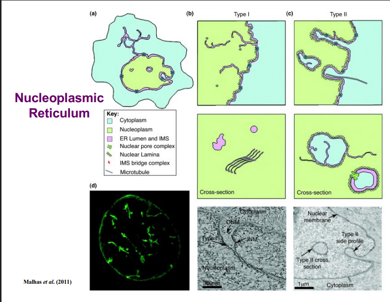
B. The Nucleus Is Not a Perfect Sphere
• Drawing the nucleus as a simple concentric circle inside a cell is misleading. In living cells, the nucleus is not a perfect sphere.
• The nuclear envelope contains numerous involutions (inward folds) called the nucleoplasmic reticulum.
• There are two types of involutions:
◦ Type I: Only the inner nuclear membrane extends inward toward the center of the nucleus.
◦ Type II: Both the inner and outer nuclear membranes invaginate together, bringing cytoplasm into the nucleus.
• These involutions are sites of active biology — they are not just structural features.
• Occasionally, involutions can pinch off entirely, creating small islands of cytoplasm within the nucleus — a phenomenon researchers are still investigating.
Functions of the Nuclear Envelope
Functions of the Nuclear Envelope
The nuclear envelope serves five major functions:
• Compartmentalization: The nuclear envelope creates a membrane-bounded compartment, separating nuclear from cytoplasmic molecules. Proteins enter via nuclear localization signals (NLS).
• Site of transport: Nuclear pore complexes mediate the import and export of molecules.
• Platform for signaling: Membrane-associated proteins on the nuclear envelope participate in intracellular signaling cascades. This connects to cell signaling, a major theme in the rest of the course.
• Structural integrity: The nuclear envelope and lamina provide physical support to maintain nuclear shape.
• Regulation of gene expression: The nuclear envelope's interaction with chromatin influences which genes are active or silent.
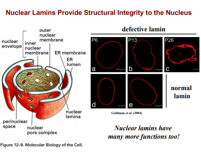
IV. Progeria: A Disease of Nuclear Envelope Defects
• Progeria is a disease of rapid aging. Individuals who are 7-10 years old may appear as elderly as 70-80 years old.
• It is caused by mutations in nuclear lamins (specifically lamin A), which disrupts the structural integrity of the nuclear envelope.
• When the nuclear envelope is deformed, the arrangement of DNA within the nucleus changes, altering gene expression.
• This disrupted gene expression affects developmental programming and accelerates the body's aging processes.
• In animal models of progeria, the nuclear envelope shows progressive distension and major malformation — visible as irregularly shaped nuclei when lamin is labeled with fluorescent markers.
• Normal nuclei have a smooth, uniform lamin distribution; progeria nuclei appear bumpy and distorted.
• Nuclear lamins have many additional functions beyond structural support — these will be revisited in a later lecture.
Organization of Chromatin in the Nucleus
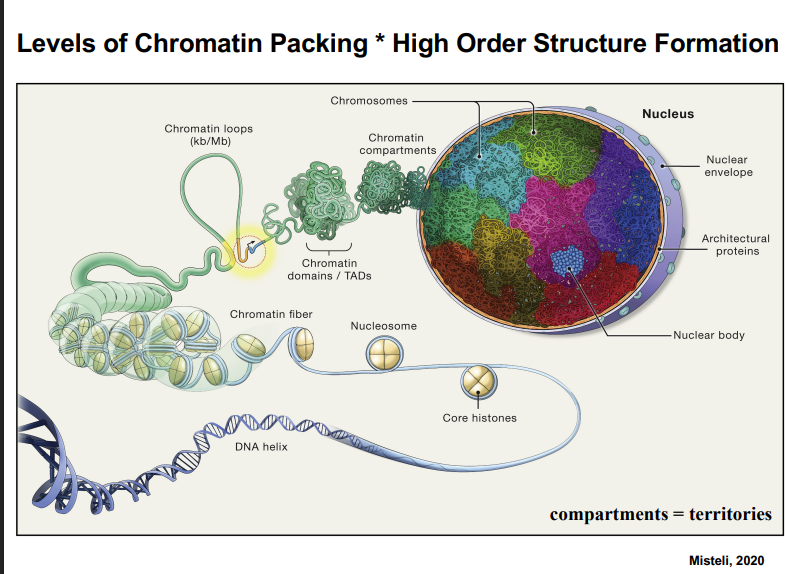
A. DNA Packing: From Double Helix to Chromatin Fiber
• DNA begins as a double-stranded helix.
• DNA wraps around histone proteins. Histones are octameric: 8 histone polypeptides form one histone unit.
• Approximately 146 base pairs of DNA wrap around one histone to form a nucleosome.
• Nucleosomes are spaced along the DNA strand — the spacing between them can be variable (often ~150 base pairs of linker DNA).
• This arrangement of nucleosomes on DNA resembles "beads on a string" and is about 10 nm in diameter.
• DNA associated with histones = chromatin. Chromatin further folds into a 30 nm chromatin fiber.
• There is broad agreement in the field on packing up to the 30 nm fiber level. Beyond this, models diverge significantly.
B. Higher-Order Chromatin Structure (Compaction)
Important distinction: Packing refers to wrapping DNA around histones. Compaction refers to higher-order organization of packed chromatin. These are not the same thing.
• 30 nm fibers interact with each other via architectural proteins to form chromatin loops.
• Loops then fold together to form chromatin domains (also called TADs — Topologically Associating Domains).
• Chromatin domains interact to form chromatin compartments.
• Chromatin compartments = chromosome territories. These two terms describe the same thing.
• A chromatin compartment is a decondensed chromosome occupying a specific region of the nucleus in a non-dividing cell. It is not membrane-bounded.
• These compartments may be thought of as biomolecular condensates — regions of phase-separated chromatin.
Chromosome Territories: History and Evidence
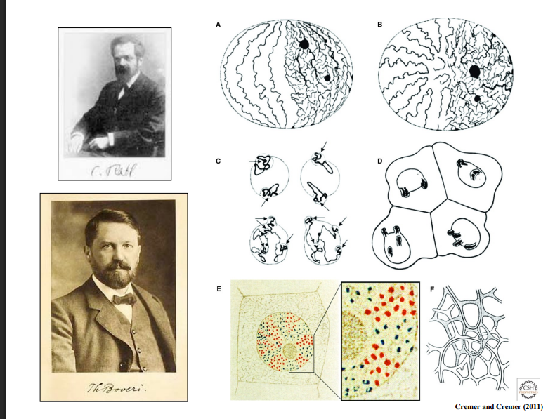
Carl Rabl (1885)
• One of the earliest observations of nuclear organization came from Carl Rabl, who studied nuclei in salamander cells using chemical stains.
• He observed large fibers in the nucleus with smaller fibers emanating from them and noted that these fibers were not intermixed like a bowl of spaghetti — they occupied distinct regions of the nucleus.
B. Theodor Boveri (~1910)
• Theodor Boveri, studying roundworm cells (Ascaris), was a pioneering cancer biologist with extraordinary observational skills.
• He observed that chromosomal material occupied only specific regions of the nucleus and coined the term "nuclear territory" (also called a nuclear compartment).
• Boveri's conceptual contributions to cancer biology were so ahead of their time that researchers today still read his original publications from over a century ago and find accurate insights with little data to support them.
• His idea of chromosome territories was largely forgotten after the electron microscope era.
C. The Electron Microscope Setback
• When electron microscopy became dominant, thin sections of cells showed nuclei that appeared largely homogeneous and gray.
• By the 1970s, the concept of nuclear territories had been essentially abandoned in the scientific community.
Experimental Revival: Microbeam Radiation Experiment (1970s)
Experimental Revival: Microbeam Radiation Experiment (1970s)
• Researchers used a UV microbeam to irradiate a specific spot within the nucleus, inducing localized DNA damage.
• Cells were labeled with radioactive tritiated thymidine, a DNA precursor. During DNA repair, cells would incorporate this label.
• Using EM autoradiography (photographic emulsion + silver grain precipitation), researchers tracked where DNA repair occurred.
• Two possible outcomes were tested:
◦ If chromosomes are intermixed (spaghetti model): radioactive repair label would appear on many chromosomes simultaneously.
◦ If chromosomes occupy territories: only one or two chromosomes (those in the irradiated zone) would show repair labeling.
• Result: When cells entered mitosis and chromosomes were examined, the repair label appeared on only a few chromosomes, not distributed broadly — supporting the territory model.
• This resurrected Boveri's century-old idea as scientifically valid.
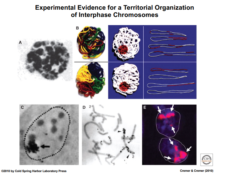
Modern Evidence: Fluorescence In Situ Hybridization (FISH)
Modern Evidence: Fluorescence In Situ Hybridization (FISH)
• FISH (Fluorescence In Situ Hybridization) uses single-stranded DNA probes complementary to specific chromosomal sequences. The probes carry fluorescent molecules.
• When probes hybridize to their target chromosome, that chromosome's location in the nucleus becomes visible under a fluorescence microscope.
• Example: A probe complementary to chromosome 8 will label chromosome 8's territory. Two signals are seen in diploid cells (two copies of each chromosome).
• Using many different fluorescent dyes simultaneously, all chromosomes can be labeled at once, producing a multicolor map of the entire nuclear interior.
• These images confirm that each decondensed chromosome in a non-dividing (interphase) cell occupies its own distinct territory.
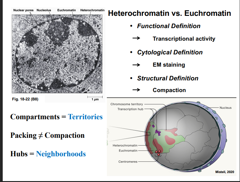
Heterochromatin vs. Euchromatin
Heterochromatin vs. Euchromatin
These terms can be defined in three ways:
A. Functional Definition
• Euchromatin: transcriptionally active chromatin.
• Heterochromatin: transcriptionally inactive chromatin.
B. Cytological Definition (based on EM staining)
• In electron micrographs, darker-staining regions of the nucleus are heterochromatin; lighter regions are euchromatin.
• Heterochromatin tends to concentrate along the nuclear envelope and around the nucleolus.
• Euchromatin is found more centrally within the nucleus.
C. Structural Definition (based on compaction)
• Heterochromatin is more highly compacted (higher-order structures).
• Euchromatin is less compacted, which allows access for transcription machinery.
• For transcription to occur, DNA must be freed from its histones — a naked DNA strand is required. This means active genes must be in a decondensed (euchromatic) state.
D. Key Spatial Observation
• Chromatin near the nuclear envelope tends to be transcriptionally inactive (heterochromatin).
• As you move from the nuclear envelope toward the center of the nucleus, transcriptional activity increases.
• This is directly relevant to progeria: when lamin is mutated and the nuclear envelope is structurally altered, chromatin that was once silenced near the envelope may become repositioned and transcriptionally activated — changing the cell's gene expression profile and contributing to premature aging.
E. Terminology Summary
• Compartments = Territories (same thing, different words)
• Packing does NOT equal Compaction (packing = DNA wrapping around histones; compaction = higher-order chromatin folding)
• Hubs = Neighborhoods (regions of the nucleus where specific activities like transcription are concentrated)
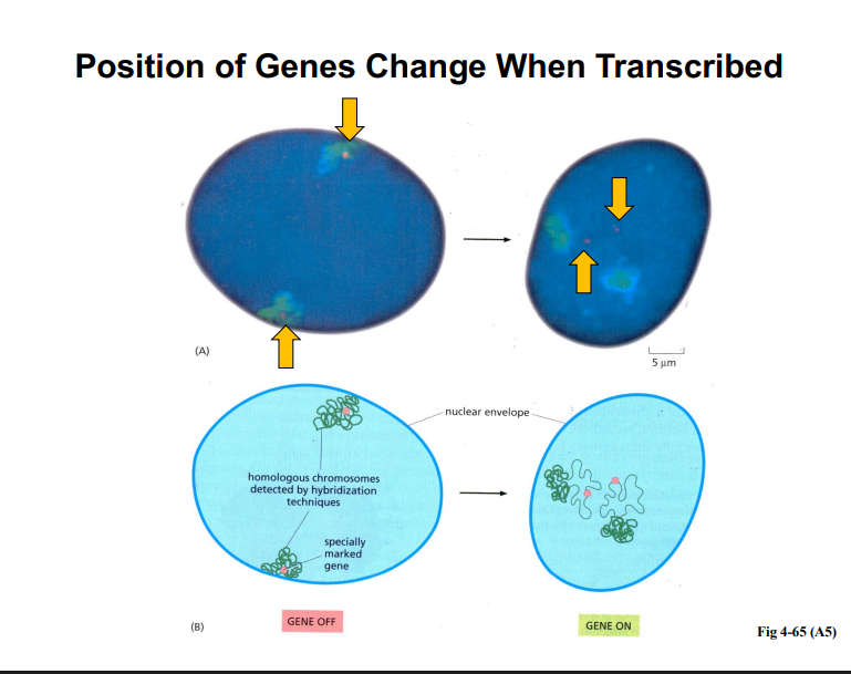
Position Effects on Gene Expression
Position Effects on Gene Expression
• The physical location of a gene within the nucleus affects whether it is transcribed.
• Genes near the nuclear envelope (heterochromatin-associated) tend to be silenced; genes moved away from the envelope and into transcriptionally active neighborhoods are expressed.
• When a gene becomes activated, its physical position within the nucleus changes — it moves away from the main body of the chromosome territory.
• This movement occurs via diffusion: loops of chromatin containing the gene diffuse away from the territory.
• However, transcribed genes tend to move to the same specific nuclear neighborhoods repeatedly, suggesting the diffusion is not entirely random. This is an active area of research.
• This is called a position effect: the physical movement of a gene into a specific nuclear location is required for or correlated with its expression.
• Transcription hubs (also called transcription neighborhoods) are regions at or near territory borders where active transcription occurs.
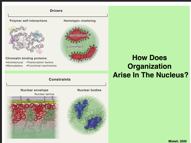
How Does Nuclear Organization Arise?
How Does Nuclear Organization Arise?
A. Drivers of Organization
• Chromatin behaves like a polymer. Polymer chemistry predicts that similar polymers self-associate (homotypic clustering).
• Heterochromatin polymers associate with heterochromatin; euchromatin polymers associate with euchromatin.
• This leads to phase separation within the nucleus — the same physical principle seen with biomolecular condensates in the cytoplasm also applies to the nucleus.
• Chromatin-binding proteins (architectural proteins, transcription factors, remodellers, and functional machineries) also drive organization by mediating specific chromatin-chromatin interactions.
B. Constraints on Organization
• Nuclear envelope constraint: Chromatin physically interacts with the nuclear lamina via protein-protein interactions. Lamina-associated proteins bind chromatin proteins, tethering heterochromatin to the inner surface of the nuclear envelope. This constrains where chromatin can go.
• Nuclear bodies constraint: Chromatin that enters nuclear bodies (neighborhoods enriched in specific proteins) becomes associated with those proteins. This also constrains chromatin positioning.
Nuclear Bodies
Nuclear Bodies
• Nuclear bodies are discrete neighborhoods within the nucleus enriched in specific proteins and DNA sequences.
• There are more than a dozen distinct types of nuclear bodies.
• Three important examples:
◦ Nucleolus: Responsible for ribosomal RNA (rRNA) production and ribosome subunit assembly.
◦ Cajal Body: Site of assembly of complexes required for mRNA processing.
◦ Speckles (Interchromatin Granule Clusters): Storage sites for complexes required for mRNA processing; found near transcription sites.
• Other nuclear bodies include Paraspeckles, PML-nuclear bodies, Histone Locus Bodies, and Gems (Gemini of Cajal Bodies), each with distinct functions.
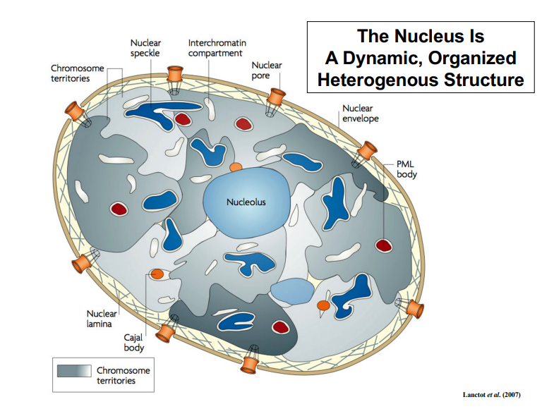
The Nucleus as a Dynamic, Organized, Heterogeneous Structure
• The nucleus should be understood not as a static compartment, but as a dynamic, organized, and heterogeneous structure.
• The concept of chromosome territories should not be thought of as having rigid, impermeable walls — DNA strands from different territories do interact with one another.
• The relationship between structure and function in the nucleus is bidirectional:
◦ Gene expression affects nuclear structure (e.g., transcription repositions chromatin).
◦ Nuclear structure regulates gene expression (e.g., position near the lamina silences genes).
• Structure does not drive gene expression; it regulates it.
• No single model fully captures how the nucleus is organized. The truth likely lies between or among multiple competing models.
Decondensed chromosomes do consistently occupy the same position in the nucleus (e.g., chromosome 8 is predictably located in a specific nuclear region).
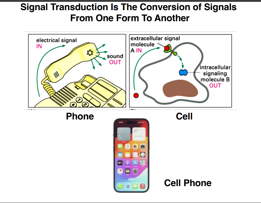
Signal Transduction — Core Concept
Signal transduction is the conversion of signals from one form to another. The classic analogy is a telephone: electrical signal comes in, audio comes out. In cells, the same logic applies — there is always an input and an output.
Input: A small molecule (could be a protein or another type of molecule) arriving at the cell
Output: Production of another small molecule or small protein inside the cell
Cells are never truly without external signals — they are constantly receiving environmental cues including temperature, pressure, and especially molecular signals.
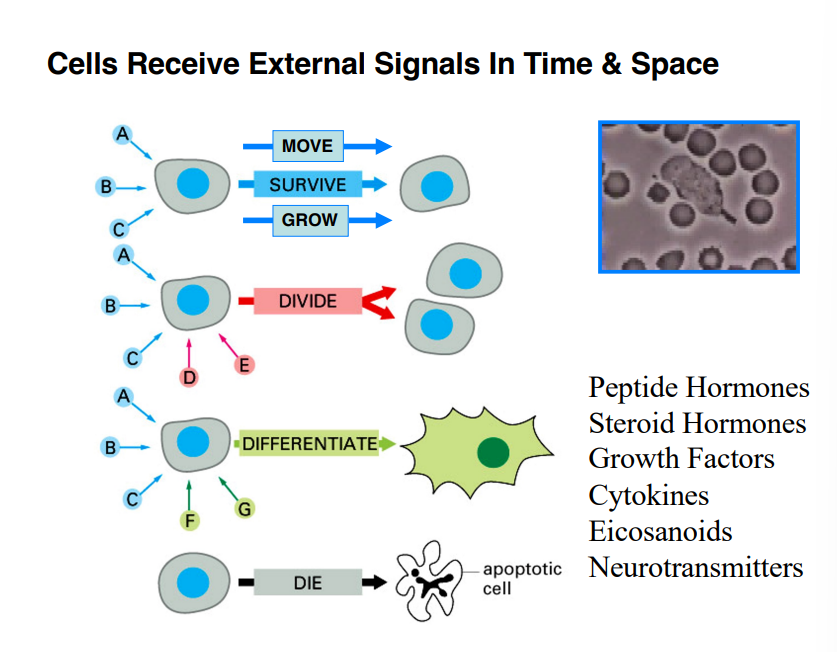
What Molecular Signals Do to Cells
A cell can receive multiple signals simultaneously, and depending on the combination, the cell responds in distinct ways:
Move, survive, or grow — signals A, B, C in the classic diagram
Divide — triggered by molecules such as growth factors or cytokines (signals D and E)
Differentiate — a cell takes on a specialized state, developing distinct structures that allow it to perform specialized functions (signals F and G)
Die (apoptosis) — in the absence of signals, a cell will undergo programmed cell death; the health and survival of a cell depends on the continuous presence of external molecular signals
A classic example of signal-driven movement is the neutrophil chasing bacteria: bacteria release molecules as they move through space, those molecules impact the neutrophil's surface, and the neutrophil moves toward the higher concentration of those molecules. This is directly relevant to cancer biology — metastatic cancer cells exploit similar chemical gradients to move through the body.
Categories of Signaling Molecules
Categories of Signaling Molecules
All of the molecules that drive the behaviors above fall into these broad categories:
Category | Key Features |
Peptide hormones | Protein-based; diverse functions |
Steroid hormones | Derived from cholesterol; lipophilic |
Growth factors | Broadly active beyond the immune system; trigger growth, division, and differentiation |
Cytokines | Associated with the immune system; modulate cell behavior |
Eicosanoids | Derivatives of arachidonic acid; heavily involved in inflammation responses |
Neurotransmitters | Small molecules; mediate signaling between neurons |
Some of these molecules are proteins; others are not. There is a great deal of overlap between categories — growth factors and cytokines in particular are used very interchangeably.

Signaling Distance — Types of Cell Signaling
Signaling Distance — Types of Cell Signaling
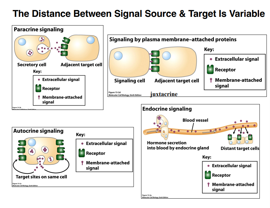
The distance between a signaling cell and its target is variable. There are four major types:
1. Paracrine Signaling
Short-distance signaling — on the order of a few micrometers
One cell releases a signal molecule; a nearby cell receives it
Example: a neutrophil tracking bacteria; the bacteria shed molecules and the neutrophil moves toward the higher concentration of those molecules
Also applies to neurons: the presynaptic neuron releases a neurotransmitter (classically acetylcholine) across a short chemical synapse, and the postsynaptic neuron binds it and responds
2. Juxtacrine Signaling
Requires direct physical contact between cells
One cell presents molecules on its surface that physically reach over and bind receptors on the adjacent cell
This type of signaling will reappear later in the course in the context of a specific mechanism of cell death
3. Autocrine Signaling
A cell signals to itself — no second cell required
The cell releases a molecule (typically through exocytosis), it washes over the cell's own surface, and binds to receptors on that same cell
Example: T cell activation in the immune system
4. Endocrine Signaling
Long-distance signaling — hormones travel half a meter or more through the bloodstream
Hormones are secreted by specific cells, enter the blood vessel, and travel to distant target cells where they exert their effects

Where Receptors Are Located
Where Receptors Are Located
Receptors are not limited to the cell surface — their location depends on the nature of the signaling molecule:
Cell-surface receptors:
Bind hydrophilic signaling molecules that cannot cross the plasma membrane
The signal is received at the surface and transduced into the cell
Intracellular receptors:
Bind lipophilic signaling molecules that can freely pass through the plasma membrane
The signaling cascade initiates inside the cell, often in the cytoplasm
Many (but not all) hormones use intracellular receptors
Example: Cortisol (stress hormone) passes through the membrane, binds an intracellular receptor protein, the cortisol-receptor complex translocates into the nucleus, binds DNA, and alters gene expression directly
Primary and Secondary Messengers
Primary and Secondary Messengers
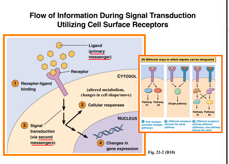
Primary messenger (ligand): The extracellular signaling molecule that binds the receptor. This is the first step of the signaling pathway.
Secondary messengers: Additional molecules produced as a result of ligand-receptor binding. These are distinct from the primary messenger, and their name simply reflects their order of appearance — they are equally important.
Secondary messengers can drive two major downstream outcomes, and both can occur simultaneously depending on the pathway:
Changes in gene expression — molecules enter the nucleus and alter transcription
Cytoplasmic responses — alterations in metabolism, organelle function, or protein structure/activity within the cytoplasm
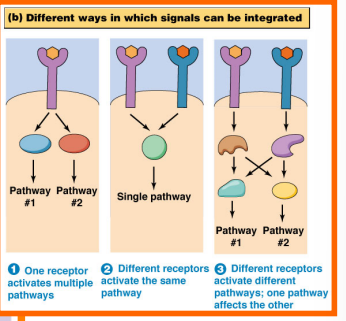
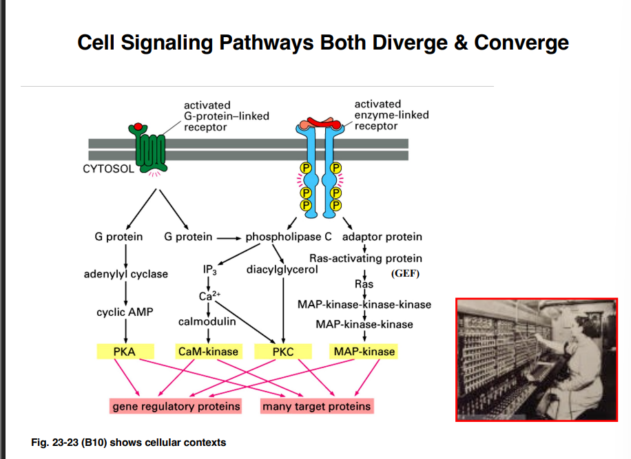
Signal Integration — How Pathways Interact
Signal Integration — How Pathways Interact
Cells integrate signals in several ways:
One receptor → two pathways: A single activated receptor can drive two distinct signaling pathways simultaneously (the "BOGO" scenario — two for the price of one molecule)
Two receptors → one output: Two different receptor types must both be activated; their downstream signals converge to produce a single integrated output
Crosstalk: Two receptors each activate separate pathways, but as the signaling cascades proceed, molecules from one pathway begin interacting with molecules from the other — and vice versa. This crosstalk is extremely common and is one of the reasons cell signaling is so complex.
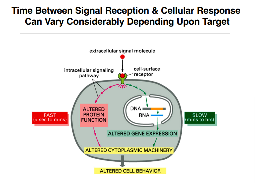
Speed of Signaling Responses
The time between signal reception and cellular response varies greatly:
Pathway Target | Speed | Example |
Gene expression changes (nucleus) | Minutes to hours (SLOW) | Transcription requires synthesis of new RNA and protein |
Protein function changes (cytoplasm) | Milliseconds to minutes (FAST) | Phosphorylation by kinases is nearly instantaneous |
Both routes ultimately result in altered cell behavior. The inputs generate specific outputs.
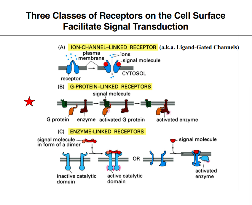
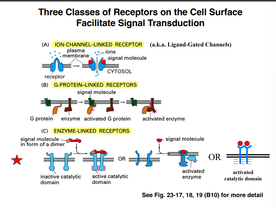
Three Classes of Cell-Surface Receptors
Three Classes of Cell-Surface Receptors
Three types of receptors on the cell surface facilitate signal transduction. Intracellular receptors (for lipophilic molecules like cortisol) are set aside for this portion of the lecture.
(A) Ion Channel–Linked Receptors (Ligand-Gated Channels)
A ligand binds to a channel protein on the cell surface
The channel opens or closes in response
Already discussed in the context of postsynaptic neurons — neurotransmitter binds the ion channel, channel opens, signaling begins
Will not be covered further here
(B) G Protein–Linked Receptors (GPCRs) ⭐(C) Enzyme-Linked Receptors ⭐
These two are the focus of this lecture.
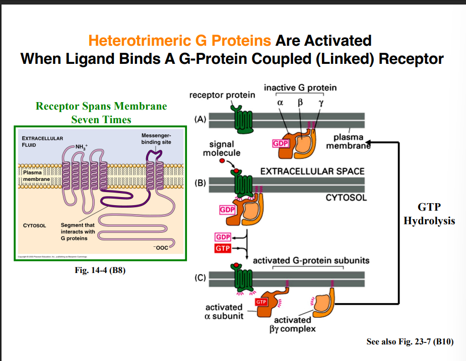
G Protein–Linked Receptors (GPCRs)
G Protein–Linked Receptors (GPCRs)Background — Two Types of G Proteins
Earlier in the course, small monomeric GTPases (20–30 kDa) were introduced — these include the Ras, Ran, Rab, and ARF families. What is discussed here is a different and distinct family: the heterotrimeric GTPases.
Hetero = the three subunits are different from each other
Trimeric = three subunits total
GTPase = the complex hydrolyzes GTP
Structure of GPCRs
GPCRs are transmembrane proteins that span the membrane seven times. Despite having very different amino acid sequences from one another, they all share this structural feature. Part of the receptor faces the extracellular space and contains the ligand-binding site.
GPCRs are an enormous and pharmacologically critical family:
The human body has just over 2,000 different GPCRs
Nearly 5% of our genome's coding sequences are devoted to GPCRs
Approximately half of all current pharmaceuticals target proteins within GPCR pathways
Mice, which rely heavily on smell, have over 1,000 GPCRs devoted exclusively to olfaction
The GPCR Activation Cycle
Step 1 — Inactive state: The heterotrimeric G protein has three subunits: α (alpha), β (beta), and γ (gamma). When inactive, GDP is bound to the alpha subunit, and all three subunits remain together as a complex.
Step 2 — Ligand binding and activation: When a ligand binds the GPCR, a conformational change occurs in the cytoplasmic domain of the receptor. This allows the receptor to bind the heterotrimeric G protein. In its activated state, the receptor functions essentially as a GEF (guanine nucleotide exchange factor) — it promotes the exchange of GDP for GTP on the alpha subunit.
Step 3 — Dissociation: Once GTP is bound to the alpha subunit, two things happen:
The G protein dissociates from the receptor
The beta and gamma subunits dissociate from the alpha subunit — but beta and gamma remain bound to each other as a βγ complex
Step 4 — Signaling by the active alpha subunit: The GTP-bound (activated) alpha subunit can now interact with and activate enzymes associated with the plasma membrane. These activated enzymes catalyze the conversion of substrates into secondary messengers.
Step 5 — Inactivation: Over time, GTP hydrolysis occurs on the alpha subunit. It returns to the GDP-bound (inactive) state and reassociates with the βγ complex, ready to restart the cycle.
Secondary Messengers — Key Molecules to Know
Secondary Messengers — Key Molecules to Know
Three categories of common secondary messengers are produced downstream of GPCR activation. Be able to distinguish their structures visually (refer to Figures 23-9 and 23-12 in Becker Chapter 23):
Category | Example(s) |
Cyclic mononucleotides | cAMP (cyclic AMP), cGMP (cyclic GMP) |
Phosphoinositides | IP₃ (inositol-1,4,5-trisphosphate) |
Diacylglycerol (DAG) | DAG |
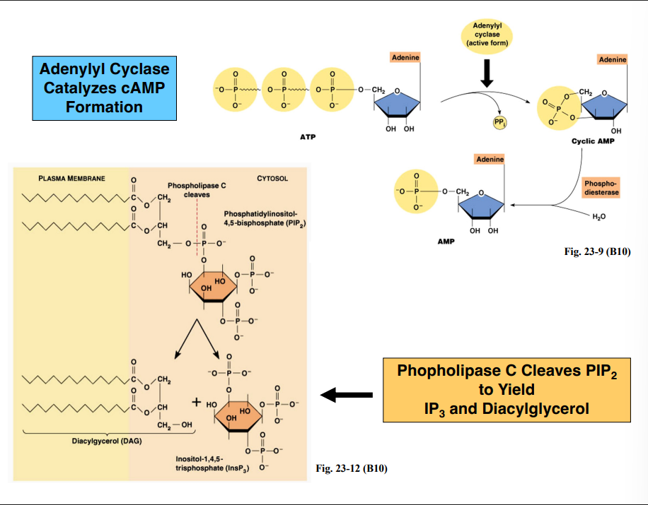
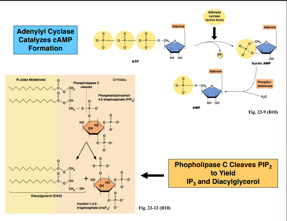
How Secondary Messengers Are Produced
How Secondary Messengers Are ProducedPathway 1 — Adenylyl Cyclase → cAMP
The activated GTP-bound alpha subunit binds and activates adenylyl cyclase (membrane-associated enzyme)
Adenylyl cyclase converts ATP → cyclic AMP (cAMP)
cAMP has a single phosphate group that forms a ring structure with the adenosine
Shutting off the signal — Phosphodiesterase:
Cells must be able to reduce cAMP levels to terminate signaling
The enzyme phosphodiesterase converts cAMP → AMP
AMP can then be recycled and recharged to become ATP again
Phosphodiesterase is the counterbalance to adenylyl cyclase (this enzyme will appear on an exam)
Pathway 2 — Phospholipase C → IP₃ + DAG
The activated GTP-bound alpha subunit can alternatively activate phospholipase C (also membrane-associated)
Phospholipase C cleaves the membrane phospholipid PIP₂ (phosphatidylinositol-4,5-bisphosphate)
The cleavage occurs at the phosphate attached to the third carbon of the glycerol backbone
This produces two secondary messengers simultaneously:
IP₃ (inositol-1,4,5-trisphosphate) — released into the cytosol
Diacylglycerol (DAG) — remains in the membrane (retains the glycerol backbone and two hydrocarbon chains)
One molecule in → two secondary messenger products out.
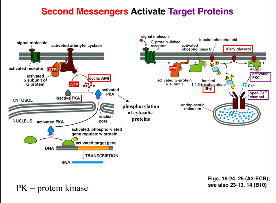
What Secondary Messengers Do — Activating Target Proteins
What Secondary Messengers Do — Activating Target Proteins
cAMP → Protein Kinase A (PKA)
cAMP activates PKA (protein kinase A)
PKA is normally a tetramer: 2 catalytic subunits + 2 regulatory subunits
2 molecules of cAMP bind to each regulatory subunit (one per subunit), causing the regulatory subunits to dissociate from the catalytic subunits
The freed catalytic subunits are now active kinases and can:
Phosphorylate cytosolic proteins (fast cytoplasmic response)
Enter the nucleus and phosphorylate gene regulatory proteins to alter transcription (slower nuclear response)
Not all PKA family members do both — it depends on the specific context and cell type
IP₃ → Calcium Release → Further Signaling
IP₃ acts as a ligand for a calcium channel embedded in the membrane of the endoplasmic reticulum (ER)
IP₃ binds the channel → channel opens → Ca²⁺ floods out of the ER into the cytosol
Cytosolic calcium concentration is normally about 0.1 micromolar — the release of ER calcium creates a large concentration gradient, making this a potent signaling event
Calcium binds to and activates various target proteins downstream
DAG → Protein Kinase C (PKC)
DAG (the second product of phospholipase C activity) remains in the membrane
DAG binds and activates PKC (protein kinase C)
PKC phosphorylates target proteins in the cytoplasm, altering their biochemical activity and protein interactions
Enzyme-Linked Receptors (Introduction)
Transmembrane proteins that pass through the membrane once (unlike GPCRs which pass seven times)
Ligand binding triggers catalytic activity — most commonly phosphorylation (though other post-translational modifications are possible)
Receptor dimerization is required for activation — ligand binding brings two receptor molecules together
Sometimes one ligand activates two receptors
Sometimes multiple ligands are needed to activate two receptors
The common requirement: the receptors must come together (cluster) to be activated
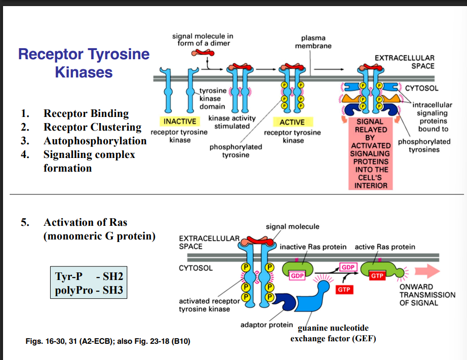
Receptor Tyrosine Kinases (RTKs) — The Largest Subclass
There are six distinct classes of enzyme-linked receptors. The largest and most important class are the receptor tyrosine kinases (RTKs):
Ligand binds to the receptors
Receptors cluster (dimerize)
Clustered receptors autophosphorylate — they add phosphate groups to themselves (on tyrosine residues)
Autophosphorylation activates the receptors
A large signaling complex assembles around the phosphorylated receptors — many proteins are recruited and activated
The details of what happens after signaling complex formation (including activation of Ras and the MAP kinase cascade) will be covered Wednesday.
Enzyme-Linked Receptors — Recap
Enzyme-Linked Receptors — Recap
These receptors are single-pass transmembrane proteins with a ligand-binding domain on the extracellular side and enzymatic activity (usually a kinase) on the cytoplasmic side. Signaling requires more than one receptor — a single isolated receptor will not signal.
• Ligand binding causes receptor clustering (at minimum, dimerization)
• The clustered receptors phosphorylate each other on their cytoplasmic domains — this is called autophosphorylation
• Autophosphorylation changes the surface chemistry of the cytoplasmic domain, enabling other proteins to dock onto the receptor
• A large signaling complex assembles on the cytoplasmic face of the receptor
Key efficiency point: The signaling complex converts a 3D diffusion problem into a 2D proximity problem. Instead of signaling molecules randomly diffusing through the cytoplasm to find each other, they are all co-localized on the receptor, immediately adjacent to one another.
Adapter Proteins, SH2 and SH3 Domains
Adapter Proteins, SH2 and SH3 Domains
An adapter protein bridges the activated receptor tyrosine kinase to a downstream molecule (a GEF — guanine nucleotide exchange factor). The adapter protein can do this because it has two distinct protein-protein interaction domains:
Domain | What It Binds |
SH2 domain | Binds phosphorylated tyrosine residues. Whenever you see a protein described as having an SH2 domain, it will be recruited to sites of tyrosine phosphorylation on an activated receptor. |
SH3 domain | Binds polyproline sequences — stretches rich in multiple proline residues. The GEF contains these polyproline sequences, so the adapter’s SH3 domain binds the GEF. |
The adapter protein is therefore simultaneously bound to the phosphorylated receptor (via SH2) and to the GEF (via SH3). This physical bridge activates the GEF, which in turn activates Ras.
Activation of Ras
Activation of Ras
Ras is a small monomeric GTPase associated with the plasma membrane. It is the 4th family of small monomeric G proteins encountered in this course (after ARF, Rab, and Ran). Like all GTPases, Ras is activated by GEFs (GDP → GTP swap) and turned off by GAP proteins (which accelerate GTP hydrolysis).
When the GEF is activated by the adapter protein, it causes Ras to exchange its GDP for GTP. GTP-bound Ras is active and initiates the MAP kinase cascade.
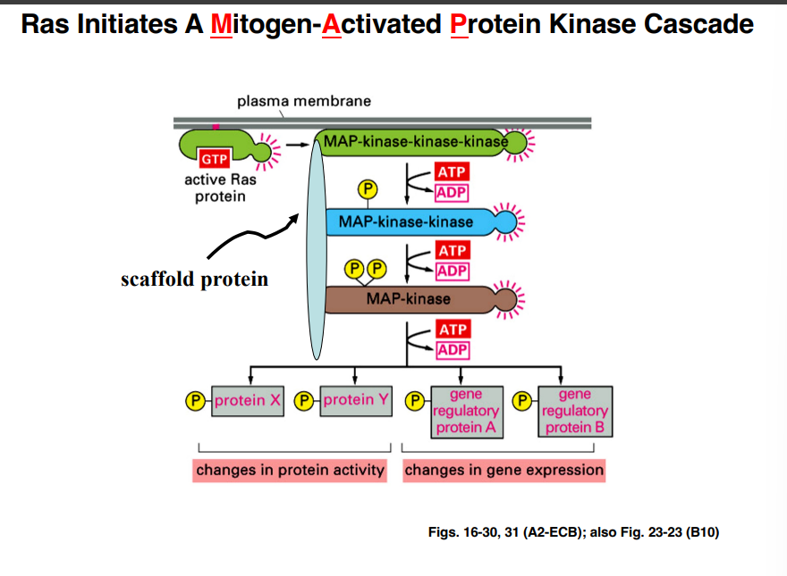
The MAP Kinase Cascade
Acronym warning: MAP here stands for Mitogen-Activated Protein. Later in the course, MAP will also stand for Microtubule-Associated Protein (cytoskeleton lectures). The professor will spell it out on exams or make the context clear.
Mitogens are molecules that stimulate cell growth and division. Active Ras-GTP triggers a three-kinase cascade:
• Active Ras activates MAP-kinase-kinase-kinase
• MAP-kinase-kinase-kinase phosphorylates and activates MAP-kinase-kinase
• MAP-kinase-kinase phosphorylates and activates MAP-kinase
• Active MAP-kinase phosphorylates downstream substrates
Downstream substrates of MAP-kinase fall into two categories:
• Cytoplasmic proteins — phosphorylation rapidly changes their activity (a fast way to alter cell function without needing new protein synthesis)
• Gene regulatory proteins (transcription factors) — phosphorylation changes their activity and alters gene expression programs
A cell may do both simultaneously depending on the cascade.
Scaffold Proteins
Scaffold Proteins
Mammalian cells have at least five different MAP kinase cascades using up to twelve kinase proteins total. Proteins can be shared across different pathways, creating potential for cross-activation and signal confusion. Scaffold proteins solve this problem.
A scaffold protein is a large protein that simultaneously binds specific kinases belonging to one particular pathway — holding the MAP-kinase-kinase-kinase, MAP-kinase-kinase, and MAP-kinase together as a pre-assembled unit.
Scaffold proteins serve two critical roles:
• Specificity: By physically grouping only the correct kinases together, the scaffold ensures the right kinases phosphorylate the right substrates and prevents inappropriate cross-activation between different MAP kinase pathways.
• Efficiency: The kinases are held right next to each other. One kinase does not have to diffuse through the cytoplasm to find the next one in the chain — again reducing the signaling problem from 3D to 2D.
The professor specifically noted that scaffold proteins are critically important yet are frequently omitted from textbook diagrams of MAP kinase cascades. This is a key point that is likely to appear on exams.
Signaling Pathways Are Not Simple On/Off Switches
Signaling Pathways Are Not Simple On/Off Switches
Signaling pathways are more like an old telephone switchboard than a light switch. Multiple inputs feed in, an operator (a protein) routes and integrates them, and a modulated output comes out. Specifically:
• Multiple signaling pathways can converge on a single protein
• That single protein integrates all the signals (both activating and inhibitory)
• A single modulated output is produced
• That output can then affect multiple processes in the cell simultaneously
This means you should think of signaling as integration and distribution of information, not simply on or off.
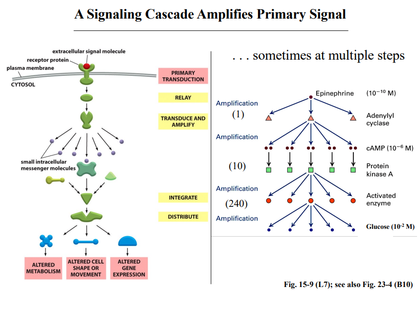
Signal Amplification
Signal Amplification
A small amount of input signal can have a profound effect on a cell. This happens because signaling cascades amplify the signal at each step — more and more molecules are produced or activated as you move downstream.
The Epinephrine Example
The professor walked through this specific amplification example in detail:
Step / Molecule | Concentration or Ratio |
Epinephrine (input) | 10⁻¹⁰ M — extremely low |
cAMP produced by adenylyl cyclase | 10⁻⁶ M — already 4 orders of magnitude higher than input |
Activated Protein Kinase A | ~10 PKA per activated adenylyl cyclase |
Next activated enzyme downstream | ~240 per PKA |
Glucose released (output) | 10⁻² M — 8 orders of magnitude above the epinephrine input |
The total amplification from input to output is 8 orders of magnitude. At each step, more molecules are produced because enzymes are catalytic — each activated enzyme can act on many substrate molecules.
The professor emphasized this is a stunning amplification. A vanishingly small hormone concentration triggers a massive metabolic response extremely rapidly.
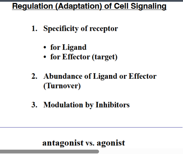
The Four Challenges of Cell Signaling
The Four Challenges of Cell Signaling
The professor framed the rest of today’s lecture around this central question: how does a cell “hear” a signal? Four things must happen:
Challenge | Explanation |
1. Distinguish the correct signal | Cells are surrounded by many molecules. The cell must recognize the specific correct ligand out of everything in its environment. This is achieved by receptor-ligand specificity. |
2. Produce the correct response | Once the correct signal is heard, the cell must produce the right intracellular response. Specificity of what proteins bind the receptor’s cytoplasmic domain ensures this. |
3. Correct amplitude | The signal must be strong enough to produce an effect. If the amplitude is too low and there is no way to boost it (e.g., through a cascade), nothing will happen. |
4. Appropriate duration | The signal must last the right length of time — not too short and not too long. Mechanisms that control ligand and effector protein turnover regulate duration. |
The professor also noted that signaling is not just a series of positive activating events. Inhibitory events are always occurring simultaneously with activating events, and there is a constant balance between the two.
Antagonists and Agonists
Antagonists and Agonists
Antagonist: A synthetic molecule (or one not naturally present in the signaling context) that competes with the natural ligand for the receptor. Antagonists bind the receptor but do not activate it, blocking the natural ligand from binding. They are blockers.
Agonist: A synthetic molecule that mimics the natural ligand and activates the receptor, often binding with greater frequency or affinity than the naturally occurring ligand. They are activators/stimulators.
The professor noted that your textbook defines these very well and recommended reviewing the definitions there.
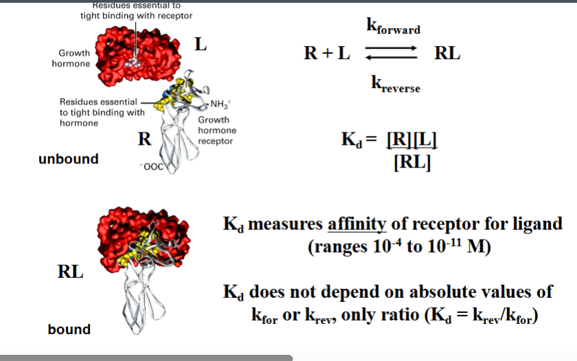
Receptor–Ligand Specificity and Molecular Complementarity
Receptor–Ligand Specificity and Molecular Complementarity
Specificity of the receptor for its ligand comes down to molecular structure. The surfaces of the two proteins have complementary shapes and chemistry — the ligand fits the receptor. This is loosely called a lock-and-key mechanism.
The professor showed the example of growth hormone binding to the growth hormone receptor. When you look at the molecular structures fitted together, they mesh extremely well.
The Dissociation Constant (Kd)
Ligand-receptor binding is reversible. The ligand is constantly binding and unbinding. The more time the ligand spends bound, the higher the affinity. This is quantified by the dissociation constant, Kd:
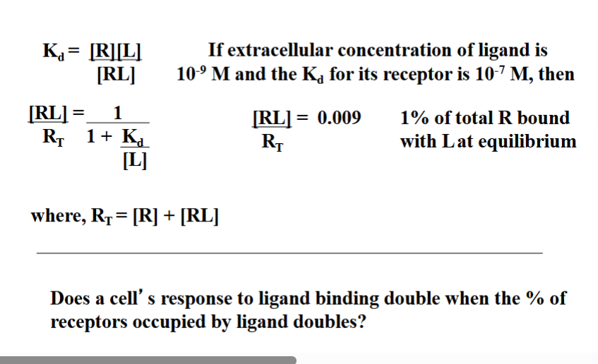
Kd = [R][L] / [RL]
Where [R] = free receptor concentration, [L] = free ligand concentration, [RL] = concentration of the receptor-ligand complex.
CRITICAL — write this in capital letters: LOWER Kd = HIGHER AFFINITY. A small Kd means the ligand spends most of its time bound (the reverse/unbinding reaction is slow relative to the forward/binding reaction). A large Kd means the ligand is weakly held and frequently unbound.
Kd values in biology range from 10⁻´ M (low affinity) to 10⁻¹¹ M (extremely high / tight binding).
Kd does not depend on the absolute values of the forward or reverse rate constants individually — only on their ratio: Kd = kᵣᵉᵥ / kᶠᵒʳ.
Binding Assays — Determining Receptor Number and Kd
How researchers actually measure the number of receptors on a cell and determine the Kd using a binding assay. The example used was insulin binding to insulin receptors.
Why Cool the Cells to 4°C?
Cells were placed at 4°C for the experiment. At low temperature, endocytosis is blocked. This prevents bound ligand from being internalized into the cell, which would falsify the measurement of surface binding.
The Three Lines on the Graph
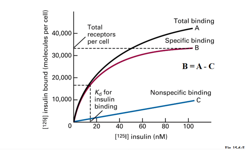
Cells were divided into dishes. Each dish received a different concentration of labeled insulin. After incubation, unbound ligand was washed away and bound ligand was measured. This produced three curves:
Line | What It Represents |
Line A — Total binding (black) | All labeled insulin bound to the cell surface at each concentration, including both receptor-bound and non-specifically bound. |
Line C — Nonspecific binding (blue) | Measured using receptor-null cells (cells that do not express the insulin receptor). Any binding in these cells has nothing to do with the receptor — it is background. |
Line B — Specific binding (red) | B = A − C. Subtracting nonspecific from total binding gives the amount of insulin specifically bound to insulin receptors. This is the biologically meaningful curve. |
Reading Receptor Number and Kd from the Graph
• The plateau of Line B (specific binding) is where all receptors on the cell surface are occupied. From the example: approximately 32,000–33,000 insulin receptors per cell.
• Kd is read from the x-axis at the ligand concentration that occupies exactly half the total receptors. In the example: when 16,000 receptors are bound, the ligand concentration on the x-axis is approximately 16–17 nM. That value is the Kd.
This is the same logic as Michaelis-Menten kinetics: KM is the substrate concentration at half-maximal enzyme velocity. Kd is the ligand concentration at half-maximal receptor occupancy. Same principle, different context.
How Many Receptors Does a Cell Typically Have?
For context the professor provided, a cell has roughly 10⁹ total proteins. About 10⁶ of those are plasma-membrane-associated. Any single receptor type typically accounts for a few thousand to ~10,000 copies, representing about 0.5–1% of all plasma membrane proteins.
Why Receptor Kd Is Greater Than Free Ligand Concentration
Why Receptor Kd Is Greater Than Free Ligand Concentration
As a general rule, a receptor’s Kd is greater than the free ligand concentration in the extracellular fluid. This is not a coincidence — it is functionally important.
The professor showed the math: if extracellular ligand concentration is 10⁻⁹ M and Kd is 10⁻⁷ M, the equation gives approximately 1% of receptors bound at equilibrium. This seems low, but it is correct and useful.
If instead the Kd were far lower than the ligand concentration, essentially 100% of receptors would always be occupied regardless of ligand concentration changes. The cell would have no ability to respond to increases or decreases in signal strength — it would be saturated at all times and have no dynamic range.
By keeping Kd above the free ligand concentration, cells maintain a wide dynamic range: they can respond proportionally across a broad spectrum of ligand concentrations.
Physiological Response Does Not Scale 1:1 with Receptor Occupancy
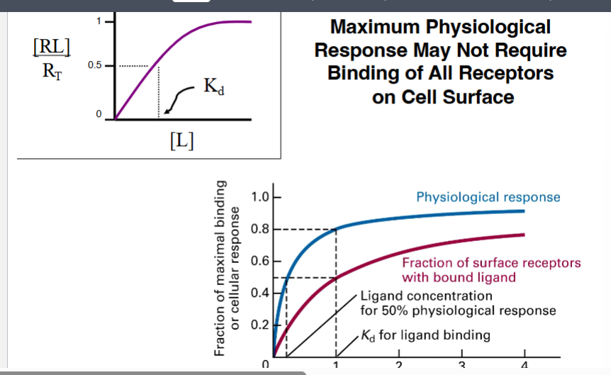
Physiological Response Does Not Scale 1:1 with Receptor Occupancy
Doubling the ligand concentration does not double the physiological response. The professor showed a graph with two curves on the same axes (ligand concentration on x-axis):
• Red line: fraction of receptors bound by ligand (receptor occupancy)
• Blue line: physiological/cellular response
The blue (response) curve rises more steeply than the red (occupancy) curve. Key observations from the graph:
• At the ligand concentration that occupies 50% of receptors (Kd = relative concentration 1), the physiological response is already approximately 80%
• A 50% physiological response is achieved at a relative ligand concentration of only about 0.2 — far less ligand than is needed to occupy 50% of receptors
This means cells respond strongly and efficiently without needing to saturate all receptors. Increasing ligand beyond a certain point produces diminishing returns on the physiological response.
Signal Desensitization — How Cells Turn Down the Signal
Signal Desensitization — How Cells Turn Down the Signal
Cells must be able to reduce or terminate signaling. The professor discussed several mechanisms:
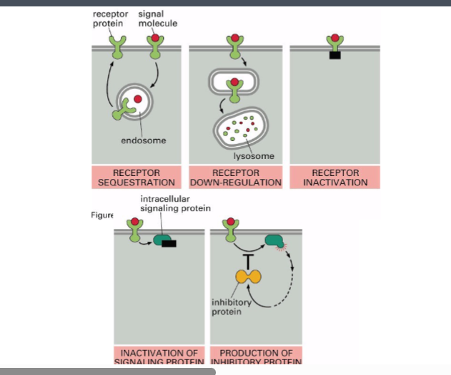
Mechanism | How It Works |
Receptor sequestration (endocytosis) | The cell endocytoses receptors from the plasma membrane into endosomes. Fewer surface receptors means less signaling. The sequestered receptors can later be recycled back to the surface via exocytosis if more signaling is needed. |
Receptor down-regulation (lysosomal degradation) | Endocytosed receptors are routed to lysosomes and destroyed rather than recycled. This permanently reduces receptor number on the surface. |
Receptor inactivation | Proteins bind the cytoplasmic domain of the receptor and physically block the formation of signaling complexes. The receptor is still on the surface but cannot signal. |
Inhibition of downstream signaling proteins | Proteins binding downstream signaling molecules (3 steps removed from the receptor or more) can inhibit an enzyme directly. Inhibition can occur anywhere along the pathway, either through protein-protein interactions or through endocytic processes. |
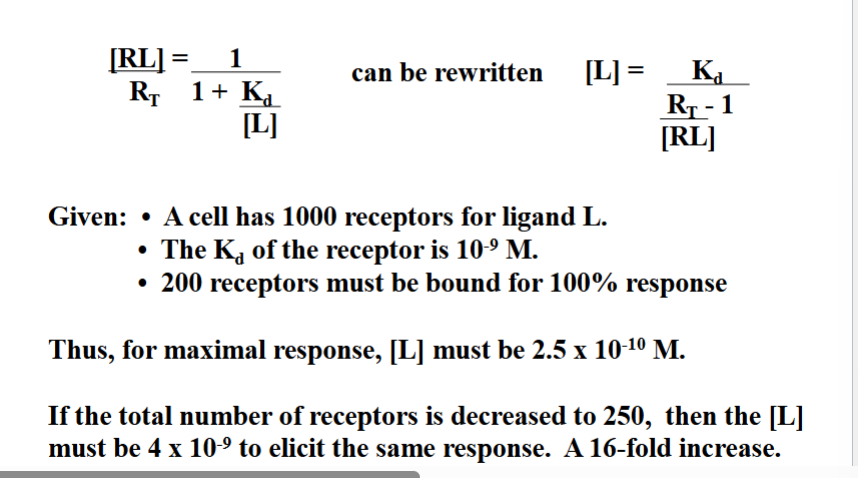
Quantitative Effect of Removing Receptors
Reducing receptor number has a disproportionately large effect on signaling sensitivity. The professor showed the math:
Starting condition: 1,000 receptors, Kd = 10⁻⁹ M, 200 receptors must be bound for a 100% response. Required ligand concentration for maximal response: 2.5 × 10⁻¹⁰ M.
After reducing receptors fourfold (from 1,000 to 250): the required ligand concentration jumps to 4 × 10⁻⁹ M. That is a 16-fold increase in required ligand — not a 4-fold increase.
Removing receptors is a very powerful desensitization mechanism because the required ligand concentration increases disproportionately. A 4-fold reduction in receptor number demands 16-fold more ligand to achieve the same response. The cell becomes far less sensitive to the signal.
Cell Signaling — Desensitization & Modulation
Cell Signaling — Desensitization & Modulation
1.1 How Cells Desensitize Themselves to Signals
Signaling must be modulated with respect to both amplitude (strength) and duration. Without active mechanisms to dampen or terminate signals, a cell would be perpetually overstimulated. Two major strategies accomplish this:
• Internalization of cell-surface receptors (receptor-mediated endocytosis)
◦ Receptors are removed from the plasma membrane and brought inside the cell. With fewer receptors available at the surface, a much higher ligand concentration is required to generate the same degree of intracellular signal — effectively turning down the volume on incoming stimulation.
• Synthesis of inhibitory proteins
◦ The cell can produce proteins that actively block steps within a signaling pathway, preventing signal from propagating further.
Both activating (stimulatory) and inhibitory pathways can operate simultaneously in the same cell. The balance between them determines the net signaling output.
G Protein-Coupled Receptors: Stimulatory vs. Inhibitory Pathways
G Protein-Coupled Receptors: Stimulatory vs. Inhibitory Pathways
Heterotrimeric G proteins are central to GPCR signaling. Their activation requires the alpha (α) subunit in the GTP-bound form. There are two functionally opposite types of alpha subunit:
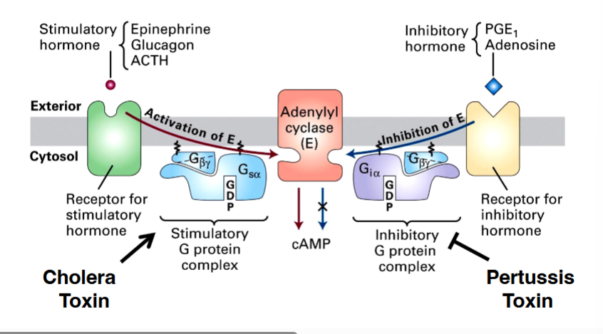
• Stimulatory pathway (Gsα)
◦ A stimulatory hormone (e.g., epinephrine, glucagon, ACTH) binds its GPCR. The receptor activates the heterotrimeric G protein, causing Gsα to exchange GDP for GTP. GTP-bound Gsα then binds and activates adenylyl cyclase, which produces cyclic AMP (cAMP). Elevated cAMP drives downstream cellular responses.
• Inhibitory pathway (Giα)
◦ An inhibitory hormone (e.g., PGE1, adenosine) binds a different GPCR. The receptor activates a different heterotrimeric G protein whose alpha subunit is Giα. When Giα is in its GTP-bound form, it binds adenylyl cyclase and inhibits it — blocking cAMP production rather than stimulating it.
◦ This opposite outcome illustrates how the identity of the proteins within a pathway — not just the pathway structure — determines whether signaling activates or suppresses a cellular response.
Pathological Disruption of G Protein Signaling: Cholera & Pertussis
Pathological Disruption of G Protein Signaling: Cholera & Pertussis
When these balanced signaling systems are disrupted by bacterial toxins, severe disease results.
• Cholera toxin — targeting intestinal epithelial cells
◦ Produced by Vibrio cholerae (first documented in human populations around the early 1800s in the Bengal region), cholera toxin is an ADP-ribosyltransferase that permanently locks Gsα in its GTP-bound, active state.
◦ Because Gsα can never hydrolyze GTP back to GDP, adenylyl cyclase is constitutively activated, causing massive, sustained cAMP production in intestinal epithelial cells.
◦ The result is a massive efflux of chloride ions and water into the gut lumen, causing the profuse watery diarrhea and rapid dehydration characteristic of cholera — the mechanism by which the disease kills.
• Pertussis toxin — targeting respiratory epithelial cells
◦ Produced by Bordetella pertussis (whooping cough), pertussis toxin also ADP-ribosylates a G protein alpha subunit, but targets Giα instead. It locks Giα in its GDP-bound, inactive (off) state.
◦ Since Giα can no longer interact with adenylyl cyclase to inhibit it, the brake on cAMP production is lost. Adenylyl cyclase runs unchecked, producing massive cAMP in respiratory epithelial cells.
◦ This leads to a massive release of fluid into the lungs, producing the hallmark hacking, whooping cough. A pertussis outbreak occurred in Virginia approximately a decade ago and persisted for one winter season — a reminder of how clinically relevant these pathways remain.
Key conceptual takeaway: Both toxins cause excessive cAMP production, but through opposite mechanisms — one locks the stimulator on, the other locks the inhibitor off. The end result is the same: loss of the normal balance between Gs and Gi signaling.
Mutant Analysis to Determine Signaling Pathway Order
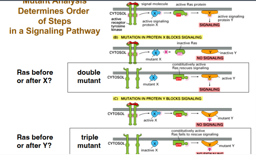
Mutant Analysis to Determine Signaling Pathway Order
Observing that two proteins interact does not establish which acts first. Genetic double- and triple-mutant analysis remains one of the most powerful tools for ordering signaling events.
The canonical pathway used in lecture (enzyme-linked receptor → adaptor to GEF/Protein X → RAS → Protein Y → downstream signaling) illustrates the logic:
• Loss-of-function mutations:
◦ If a loss-of-function mutation in Protein X (the GEF) blocks signaling entirely, that protein is required for signal propagation. This can be detected in a cell-based assay.
• Constitutively active (dominant) mutations:
◦ A constitutively active mutation locks the protein in its active form permanently — it is always "on." For RAS, a specific point mutation locks it in the GTP-bound (active) state.
• Double mutant logic (Is RAS before or after Protein X?):
◦ Combine constitutively active RAS + loss-of-function Protein X. If signaling still occurs, RAS must act downstream of (after) Protein X — because active RAS bypasses the block. If signaling is still absent, RAS acts upstream of (before) Protein X.
• Triple mutant logic (Is Protein Y before or after RAS?):
◦ Add a loss-of-function Protein Y to the constitutively active RAS + loss-of-function Protein X background. If signaling is now abolished, Protein Y must act downstream of RAS — because even constitutively active RAS cannot bypass a downstream block at Protein Y.
This epistasis analysis assigns each protein to a position in the hierarchy, establishing the sequence of events without needing to directly observe molecular interactions in real time.
Membrane-Associated Signaling: Microvesicles and Exosomes
Membrane-Associated Signaling: Microvesicles and Exosomes
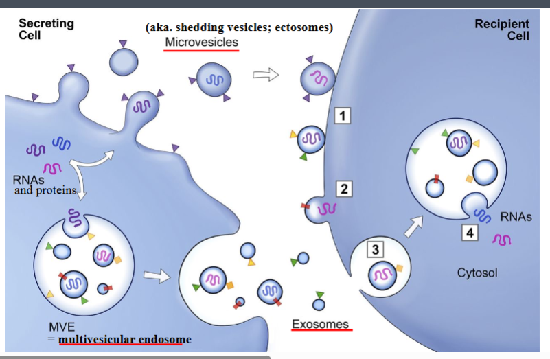
Beyond secreted small molecules and direct cell-cell contact, cells can signal by releasing membrane-bounded vesicles carrying biological cargo. There are two major classes:
• Microvesicles (also called shedding vesicles or ectosomes)
◦ Formed by direct outward budding of the plasma membrane. The term "microvesicle" has largely replaced older synonyms.
◦ Diameters range from approximately 100 nm up to nearly 1 micrometer, depending on cell type.
◦ First observed in the 1940s, their functional significance was not understood for decades.
◦ Cargo is specific — particular proteins and RNA molecules are selectively incorporated, not random cytosolic contents.
◦ Upon reaching a target cell, microvesicles can (a) fuse directly with the plasma membrane to release contents into the cytoplasm, or (b) be internalized by endocytosis, passing through early endosomes → late endosomes before contents are released.
• Exosomes
◦ Smaller than microvesicles — typically 50–200 nm in diameter.
◦ Not derived from the plasma membrane of the source cell. Instead, they form inside a large intracellular compartment called the multivesicular endosome (MVE): the inner membrane of the MVE invaginates inward and buds off to create small internal vesicles. When the MVE fuses with the plasma membrane via exocytosis, these internal vesicles are secreted as exosomes.
◦ Like microvesicles, their cargo (proteins, mRNA, other molecules) is specifically sorted — not a random sample — and research is actively investigating the molecular basis of this sorting.
• Why it matters — the concept of non-autonomous cells:
◦ This mode of signaling challenges the classic view of the cell as a completely autonomous unit. When mRNA from one cell is delivered to and translated in another, genetic information has crossed cellular boundaries — cells are not always self-contained.
• Clinical relevance — biomarkers for disease:
◦ Microvesicles and exosomes carry unique molecular signatures (proteins, nucleic acids) that reflect the state of the cells that produced them. A blood sample can be analyzed for specific exosomal or microvesicular proteins to detect susceptibility to, or presence of, particular diseases. This has driven significant research over the past decade into identifying appropriate biomarkers for diagnostic purposes.
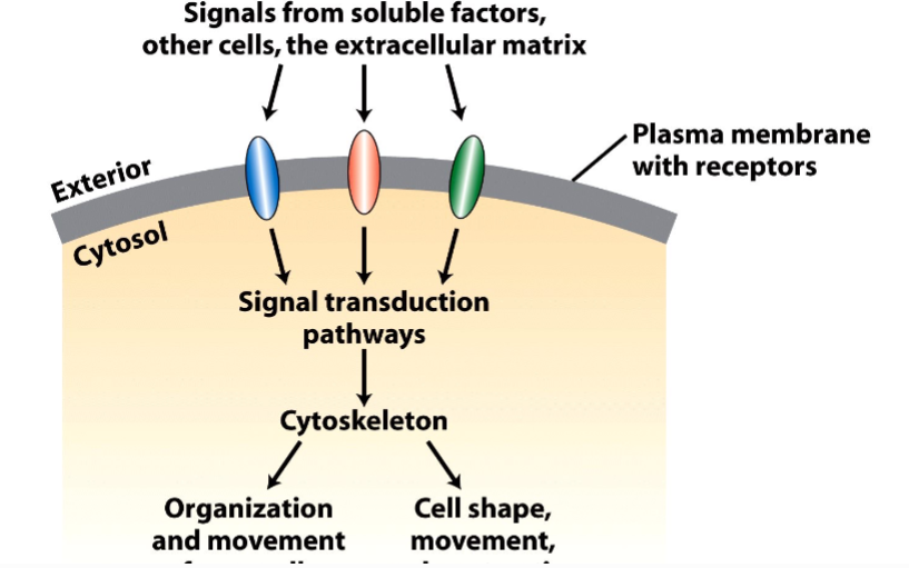
The Cytoskeleton
Why the Cytoskeleton Matters
Signal transduction pathways ultimately have to drive physical outcomes in the cell — organelle movement, changes in cell shape, directed cell migration. The cytoskeleton is the structural and mechanical apparatus that executes these outcomes. It is also directly relevant to cancer biology: cancer cells exploit cytoskeletal machinery to migrate to locations where they should not be (metastasis).
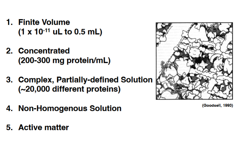
Physical Properties of the Cytoplasm
Physical Properties of the Cytoplasm
Before describing the cytoskeleton, it is critical to understand what the cytoplasm is actually like — it is not a dilute aqueous solution like a laboratory test tube.
• Finite volume
◦ Cytoplasmic volume ranges from about 1 × 10⁻¹¹ µL (in small prokaryote-sized compartments) to 0.5 mL in the largest cells. Small volumes mean that even a single molecule can represent a biologically meaningful concentration — in an E. coli cell, one molecule equals approximately 1 nM. In a mammalian cell, ~1,000 molecules are needed for the same 1 nM concentration. Small changes in molecule number can profoundly alter biochemistry.
◦ Practical example: a secretory vesicle has a volume of roughly 5 × 10⁻⁷ picoliters. Within such a compartment, adding just 48 protons shifts the pH by a full unit — demonstrating how few molecules are needed to produce significant chemical changes in small compartments.
• Extremely concentrated
◦ Protein concentration in the cytoplasm is 200–300 mg/mL. For comparison, a 1 mg/mL protein solution is already considered concentrated for biochemical experiments in a test tube. The cytoplasm contains two orders of magnitude more protein — it is extraordinarily crowded.
• Complex and partially defined
◦ Roughly 17,000–20,000 different proteins are present at any given moment in a mammalian cell, constantly undergoing post-translational modifications. This composition is impossible to define precisely at any single instant in time.
• Non-homogeneous
◦ Proteins are not evenly distributed throughout the cytoplasm. Different proteins are enriched in different regions, creating spatial organization that is functionally important.
• Active matter
◦ Molecular motion in the cytoplasm far exceeds what would be produced by simple diffusion alone. Biochemical reactions release heat, and motor proteins consuming ATP actively stir the cytoplasm by transporting organelles and chromosomes. The cytoplasm is dynamically agitated.
• Both gel-like and solution-like
◦ The cytoplasm exhibits properties of both a gel and a liquid depending on the conditions and scale of observation. This duality becomes especially relevant when studying amoeboid cell motility.
• Viscoelastic
◦ A purely elastic material (like a spring) deforms and immediately snaps back to its original shape. A purely viscous material (like fluid in a dashpot/piston) deforms slowly and barely returns. The cytoplasm is viscoelastic — it can be rapidly deformed, but recovery to its original shape takes time. This behavior is directly tied to the protein filament networks (the cytoskeleton) within it.
• Low microviscosity / high macroviscosity
◦ Particles smaller than ~10 nm in diameter diffuse freely through the cytoplasm (low microviscosity). Particles larger than ~10 nm experience dramatically reduced mobility and are essentially trapped (high macroviscosity).
◦ This observation, from microinjection experiments tracking magnetic particles, led directly to the discovery that a structural lattice must exist inside the cell to obstruct large particle movement.
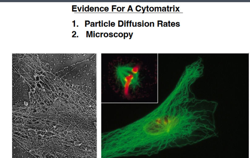
Evidence for a Cytomatrix (Cytoskeleton)
Evidence for a Cytomatrix (Cytoskeleton)
Keith Porter (University of Pennsylvania, Nobel laureate) pioneered evidence for an intracellular protein lattice, initially called the microtrabecular lattice — a term now replaced by cytoskeleton/cytomatrix. His approach:
• Detergent extraction + electron microscopy:
◦ Cells were washed with a non-ionic detergent (which solubilizes all membranes without disrupting protein-protein interactions). When the remaining material was examined by electron microscopy, a net-like lattice of fibers was visible — the structural framework of the cell.
• Particle diffusion experiments:
◦ Large injected beads were not moving freely — they were physically hindered by the protein filament lattice, confirming the structural lattice identified by electron microscopy was real and present in living cells.
• Fluorescence microscopy:
◦ The development of fluorescent probes for specific cytoskeletal proteins allowed visualization of these filament networks in living cells — confirming the structures seen in fixed and detergent-extracted preparations were not artifacts.
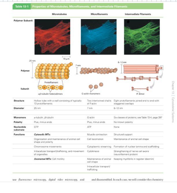
Three Filament Networks of the Cytoskeleton
Three Filament Networks of the Cytoskeleton
Mammalian cells contain three distinct cytoskeletal systems, all of which can coexist in the same cell simultaneously. They are distinguished by their diameter and protein composition (see Table 13-1 in the textbook):
• Microtubules — 25 nm diameter
◦ Found primarily in the cytoplasm. Assembled from tubulin subunits. Responsible for chromosome segregation in mitosis and meiosis.
• Intermediate filaments — ~10 nm diameter
◦ Found in both cytoplasm and nucleus. Nuclear lamins (which form the nuclear lamina lining the inner face of the nuclear envelope) are intermediate filament proteins. Their diameter (roughly between 7 and 25 nm) is the basis for the name "intermediate."
• Microfilaments (actin filaments) — 7 nm diameter
◦ Found primarily in the cytoplasm. Small actin-like structures are also present near the nuclear lamina, where they appear to contribute to nuclear envelope support and function — though no full actin lattice exists throughout the nucleus.
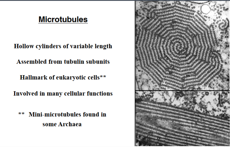
Microtubules: Structure and Composition
Microtubules are hollow cylindrical polymers, 25 nm in diameter, with variable length. Changes in microtubule length are central to many biological processes.
Tubulin Subunits
• Each tubulin subunit is a heterodimer composed of α-tubulin and β-tubulin — two distinct polypeptides that are permanently and irreversibly associated with each other. The word "tubulin" or "tubulin subunit" in cell biology always refers to this α/β heterodimer.
• Each heterodimer binds two GTP molecules:
◦ One GTP sits at the α/β interface and never hydrolyzes — it is structural.
◦ One GTP is bound to the β-subunit and can be hydrolyzed to GDP + Pi. This hydrolysis event is central to microtubule dynamic instability (discussed in subsequent lectures).
• Importantly, tubulin is classified as a G protein in the biochemical sense (it binds and hydrolyzes guanine nucleotides), but it is not a signaling G protein in the way heterotrimeric or monomeric Ras-like GTPases are.
Protofilaments and Microtubule Assembly
• Heterodimers associate end-to-end to form linear chains called protofilaments. The α-subunit of one dimer contacts the β-subunit of the adjacent dimer.
• Thirteen protofilaments arrange side-by-side in a circle to form one microtubule — creating the hollow tube that is visible in cross-section electron micrographs as 13 individual circles, each representing the end of one protofilament.
Polarity: Plus and Minus Ends
• Because α/β heterodimers are asymmetric and always align in the same head-to-tail orientation, microtubules have intrinsic polarity — the two ends are structurally and chemically distinct:
◦ Plus end (+): β-tubulin is exposed at this end. This end grows faster and is the primary site of dynamic instability.
◦ Minus end (−): α-tubulin is exposed at this end. In cells, this end is typically anchored or stabilized.
◦ Note: plus/minus terminology has no relationship to electrical charge or magnetism — it is simply a naming convention to distinguish the two ends.
Higher-Order Microtubule Structures
• Singlet: a single microtubule (13 protofilaments).
• Doublet: two microtubules fused together (A-tubule complete, B-tubule sharing the A-tubule wall). Found in cilia and flagella.
• Triplet: three fused microtubules. Found in centrioles and basal bodies.
Main Functions of Microtubules
• Chromosome segregation during mitosis and meiosis — mitotic spindle microtubules attach to chromosomes and pull them apart.
• Transport of membrane-bounded organelles — microtubules serve as tracks along which motor proteins carry vesicles and organelles.
• Cell motility and morphogenesis — microtubules are involved in directing and enabling cell movement and shape changes.
• Ciliary and flagellar beating — the 9+2 axonemal array of doublet microtubules powers the beating of cilia (e.g., in the respiratory tract) and eukaryotic flagella (e.g., sperm).
Microtubules Are Not Exclusively Eukaryotic
Microtubules Are Not Exclusively Eukaryotic
For most of cell biology's history, microtubules were considered a defining hallmark of eukaryotic cells. This has been revised:
• Mini-microtubules have been discovered in certain members of the Asgard archaea — a phylum of archaea that sits on the same evolutionary branch as eukaryotes (distinct from bacteria).
• These archaeal microtubules are smaller in diameter than eukaryotic microtubules and are built from a protein whose sequence is intermediate between bacterial tubulin homologs and eukaryotic tubulin.
• The working hypothesis is that these Asgard archaeal structures represent the evolutionary precursors of the more elaborate eukaryotic microtubule system — ancestral microtubules that were further elaborated along the eukaryotic lineage.
Coming up: The lecture will continue with microtubule assembly dynamics (critical concentration, dynamic instability, GTP cap mechanism) and microtubule-associated proteins (MAPs). Reading: Becker Ch. 13.1–13.2 (pp. 359–370).
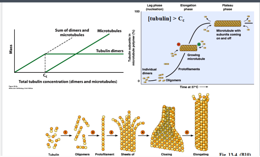
Microtubule Structure and Composition
A. Subunit Composition
Microtubules are hollow cylindrical polymers assembled from protein subunits. The fundamental building block is a heterodimer composed of two related proteins: alpha-tubulin and beta-tubulin. These two polypeptides have an extremely high affinity for one another, meaning that when the term "tubulin subunit" or "tubulin dimer" is used, it always refers to the alpha-beta pair together — never an individual monomer in isolation.
• Alpha-tubulin and beta-tubulin together form the heterodimer (the actual microtubule subunit).
• Heterodimers assemble head-to-tail into linear chains called protofilaments. In a protofilament, alpha always faces one direction and beta faces the other — this asymmetry is critical.
• Typically 13 protofilaments associate laterally (side-by-side) via non-covalent interactions and curve to close into a hollow tube — the microtubule. The number 13 is typical but not invariant.
B. Higher-Order Microtubule Structures
Not all microtubules in a cell are single, independent tubes. Depending on location and function, microtubules can be fused together into doublet or triplet configurations where they share some protofilaments in common:
• Singlet microtubules: The standard 13-protofilament hollow cylinder. Found throughout the cytoplasm.
• Doublet microtubules: Two microtubules fused together, sharing a wall of protofilaments. Found specifically in cilia and flagella of eukaryotic cells.
• Triplet microtubules: Three fused microtubules (A, B, and C tubules) sharing protofilaments. Found exclusively in centrioles and basal bodies.
C. Microtubule Polarity: Plus and Minus Ends
Because heterodimers always assemble head-to-tail, a protofilament is structurally asymmetric — one end terminates with a beta-tubulin polypeptide and the other terminates with an alpha-tubulin polypeptide. This asymmetry is inherited by the entire microtubule, giving it two chemically and structurally distinct ends:
• Plus end (+): The end where the outermost subunit exposes a beta-tubulin polypeptide. This end has a lower critical concentration for assembly and is where the vast majority of important biology occurs.
• Minus end (−): The end where alpha-tubulin is exposed. In most cellular contexts, the minus end is relatively inert biologically. It is often anchored or capped at the microtubule organizing center.
• Important note: The plus/minus nomenclature has nothing to do with electrical charge or magnetism. It is purely a naming convention to distinguish the two structurally different ends.
II. Main Functions of Microtubules
Microtubules are involved in four major cellular processes:
• Chromosome segregation during mitosis and meiosis
• Transport of membrane-bounded organelles throughout the cytoplasm
• Cell motility and morphogenesis (shaping the cell)
• Ciliary and flagellar beating
Microtubule Assembly and Polymerization Kinetics
A. On-Rate, Off-Rate, and Critical Concentration
Microtubule assembly can be described by two rate constants:
• k-on: The rate constant describing the addition of free tubulin subunits onto the end of a growing microtubule (polymer).
• k-off: The rate constant describing the loss of tubulin subunits from the polymer back into the free subunit pool.
• Critical concentration (Cc): Defined as k-off / k-on. At this concentration, the rate of subunit addition equals the rate of subunit loss — the system is at equilibrium and net polymer mass does not change.
On a graph of polymer mass versus total tubulin concentration:
• Below Cc: subunits come off polymer faster than they add on; polymer disassembles.
• At Cc: equilibrium — no net change in polymer mass.
• Above Cc: subunits add faster than they come off; more polymer forms. The mass of free dimers in solution plateaus (stays flat) while total polymer mass increases.
Relationship between critical concentration and KD: The critical concentration resembles and is sometimes used as an approximation of the dissociation constant (KD) — sometimes called an "apparent KD." However, they are conceptually distinct. Critical concentration describes the balance point between assembly and disassembly of a polymer, while KD describes the binding affinity between two individual molecules or subunits. The distinction will become more important in subsequent lectures.
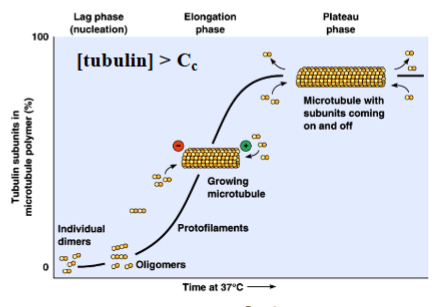
Nucleation and Kinetics of Polymerization (Lag, Elongation, Plateau Phases)
When microtubule polymerization is measured over time at concentrations above Cc, three distinct phases are observed:
• Lag (nucleation) phase: Initially, very few subunits are incorporated into polymer. Free dimers must collide randomly and begin to associate, forming oligomers. Oligomers elongate into short protofilaments. Protofilaments establish lateral contacts with each other to form sheets. The sheets curve and close into a hollow tube — the nascent microtubule. This entire process is slow because it depends on random collision and self-organization.
• Elongation phase: Once a short, stable microtubule exists (a "seed" or "nucleus"), it provides a pre-established platform onto which additional subunits can rapidly and continuously add. This phase is characterized by a steep increase in the percentage of tubulin in polymer form over time.
• Plateau (steady-state) phase: As the free tubulin pool is consumed, it becomes harder for subunits to find the end of a microtubule. The rate of addition slows and approaches the rate of loss, reaching a new steady state. Net polymer mass stops increasing.
Key insight: The rate-limiting step in microtubule assembly is nucleation — getting the initial polymer started. Once a template exists, elongation is rapid. This is why cells use nucleating proteins (like gamma-TURC) to bypass the slow spontaneous nucleation step.
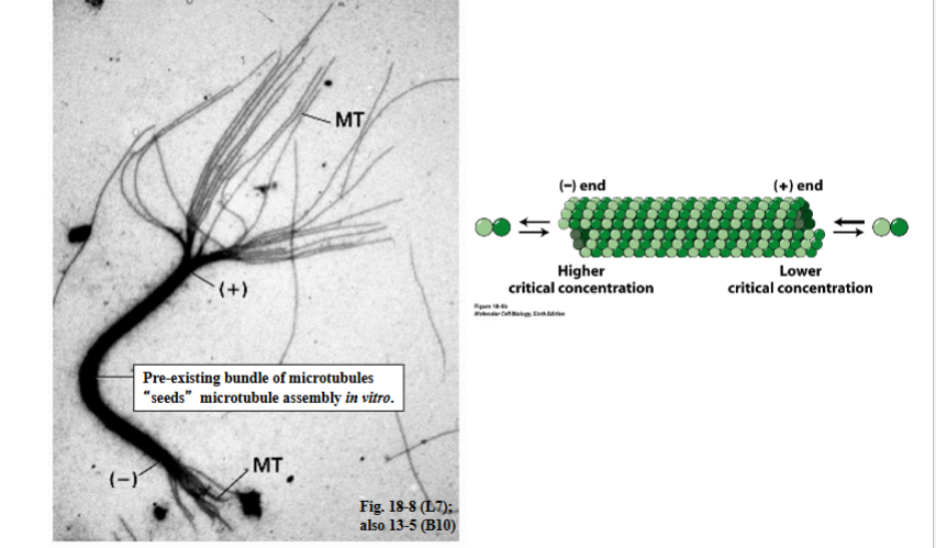
Asymmetric Growth: Plus vs. Minus End Critical Concentrations
Asymmetric Growth: Plus vs. Minus End Critical Concentrations
Experimental evidence demonstrates that the two ends of a microtubule do not grow at the same rate. In the classic "seeding" experiment, a stable bundle of microtubules is placed into a tubulin solution above Cc. New microtubule growth is substantially greater at the plus ends than at the minus ends — in fact, the minus end shows minimal growth under these conditions.
• The plus end has a lower critical concentration for assembly — meaning subunits start incorporating at lower concentrations, and the on-rate is faster relative to the off-rate.
• The minus end has a higher critical concentration — it requires a higher tubulin concentration to sustain net growth, so under typical physiological conditions it is the "quiet" end.
• This difference in critical concentrations at each end explains why nearly all the important biology of microtubules happens at the plus end.
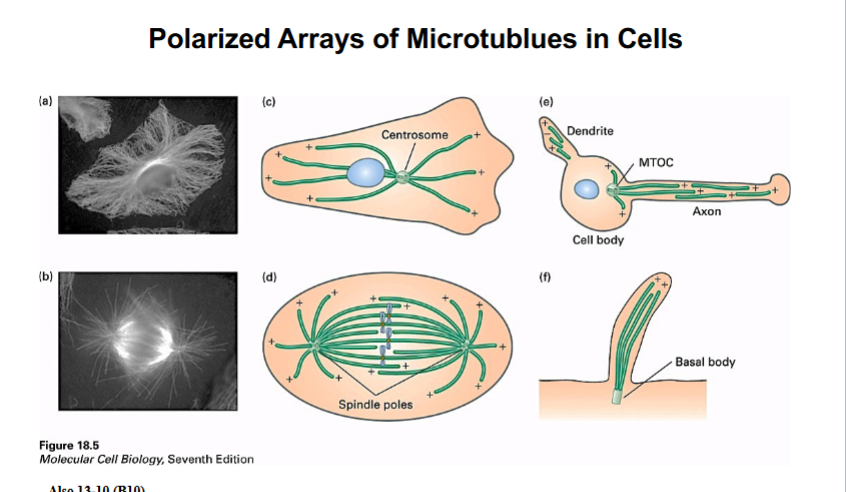
Polarized Arrays of Microtubules In Cells
Polarized Arrays of Microtubules In Cells
In living cells, microtubules are not randomly oriented. They form "polarized arrays" — organized arrangements in which the plus ends and minus ends are consistently positioned in specific locations relative to cell architecture. This organization is essential for directed transport and other functions.
• Typical mammalian interphase cell: Minus ends are anchored near the center of the cell at the centrosome (microtubule organizing center). Plus ends radiate outward toward the plasma membrane.
• Mitotic spindle: Plus ends of spindle microtubules point inward, toward the condensed chromosomes (or toward the cell equator). Other microtubules point outward toward the plasma membrane.
• Cilia and flagella: Plus ends are located at the tip, distal from the cell body. Minus ends are anchored at the basal body near the cell surface.
• Axons (neurons): Plus ends point away from the cell body, toward the axon terminus. This uniform polarity is critical for directional transport of vesicles and organelles.
• Dendrites (neurons): The exception — plus and minus ends are intermixed in both orientations throughout the dendrite. This mixed polarity distinguishes dendritic microtubule organization from axonal organization.
This polarized arrangement has profound consequences for how organelles are distributed and transported, as molecular motors recognize the directionality of microtubules to move cargo in specific directions.
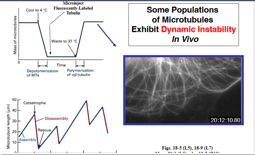
Dynamic Instability
Dynamic Instability
A. Discovery and Description
Early biochemical measurements of microtubule assembly showed that above Cc, the mass of polymer increased and then plateaued. The naive interpretation was that microtubules grew to a certain length and then simply sat there at steady state. This view turned out to be incorrect.
When researchers began combining fluorescence microscopy with fluorescently labeled tubulin in live cells or in vitro systems, they observed something unexpected: individual microtubules are not static at steady state. Instead, some microtubules are actively growing while neighboring microtubules are actively shrinking — simultaneously, within the same cell or reaction.
This behavior is called dynamic instability. It is a property of individual microtubules, not of a population average. The two key events that define dynamic instability are:
• Catastrophe: A sudden, rapid switch from a growing or paused microtubule to rapid depolymerization. The microtubule shrinks quickly — but it does not necessarily disappear entirely. Ex. Catastrophen short and more dynamic
• Rescue: After a catastrophe event, a depolymerizing microtubule can switch back to a state of growth. The microtubule begins elongating again from its shortened state.
Dynamic instability occurs primarily at the plus end of the microtubule. The kymograph (a stacked time-series image used in fluorescence microscopy) is a powerful tool for visualizing this behavior. In a kymograph, time is on the y-axis and distance along the microtubule is on the x-axis, allowing one to see growth, pause, catastrophe, and rescue events in a single image.
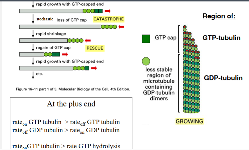
Molecular Mechanism: The GTP Cap Model
Molecular Mechanism: The GTP Cap Model
Dynamic instability is explained by the nucleotide state of tubulin subunits within the microtubule. Tubulin is a GTPase — it binds GTP, and the beta-tubulin subunit can hydrolyze GTP to GDP after incorporation into the polymer. Alpha-tubulin also binds GTP, but that GTP is not hydrolyzed and is essentially irrelevant to the dynamics.
There are two populations of tubulin heterodimers to track:
• GTP-bound tubulin (dark green in slide diagrams): The free subunit form. GTP-tubulin has favorable assembly kinetics.
• GDP-bound tubulin (light green in slide diagrams): Tubulin whose beta-subunit GTP has been hydrolyzed after incorporation. GDP-tubulin has unfavorable assembly kinetics.
The key kinetic relationships at the plus end are:
• Rate-on of GTP-tubulin > Rate-off of GTP-tubulin: GTP-tubulin adds to the plus end faster than it comes off. Net addition occurs when GTP-tubulin is available.
• Rate-off of GDP-tubulin > Rate-on of GDP-tubulin: GDP-tubulin dissociates from the plus end faster than GDP-tubulin can re-add. GDP-tubulin destabilizes the end.
• Rate-on of GTP-tubulin > Rate of GTP hydrolysis: This is the critical relationship. The rate at which new GTP-tubulin adds to the end slightly exceeds the rate at which GTP is hydrolyzed on recently-added subunits. This creates a slight temporal delay before hydrolysis converts the newest subunits to GDP-tubulin.
The GTP Cap:
Because hydrolysis lags slightly behind addition, the very tip of a growing microtubule is always capped by a small region of recently added GTP-tubulin subunits. This region is called the GTP cap. The GTP cap stabilizes the plus end, allowing continued growth.
The body of the microtubule, behind this growing tip, consists predominantly of GDP-tubulin — the hydrolysis product of earlier-added subunits. Most of the microtubule lattice is therefore in the "unstable" nucleotide state, but is stabilized by being deeply embedded within the polymer lattice rather than exposed at the end.
How Catastrophe Occurs
As a microtubule grows longer, it consumes the free tubulin pool. The concentration of free GTP-tubulin subunits drops, so the intervals between new subunit additions become longer. If the gap between additions is long enough, all of the most recently added subunits have time to hydrolyze their GTP to GDP before the next GTP-tubulin arrives.
When the GTP cap is lost — meaning GDP-tubulin is now exposed at the very tip of the plus end — the end becomes unstable. GDP-tubulin dissociates rapidly. The protofilaments at the end begin peeling apart (curling outward), and rapid depolymerization ensues. This is catastrophe.
How Rescue Occurs
After catastrophe, the free GTP-tubulin pool has been replenished (because subunits rapidly exchange their GDP for GTP when free in solution). With a now-sufficient concentration of GTP-tubulin, the probability of re-capping the plus end increases. When new GTP-tubulin adds to the shrinking end faster than it is lost, the GTP cap is reestablished, and the microtubule switches back to growth — this is rescue.
An important nuance in current research: The exact nature of the GTP cap (how many GTP-tubulin subunits are needed, their structural arrangement) is still an active area of investigation. The challenge is reconciling the chemical/biochemical view of microtubule dynamics with the material science / structural biology view of the microtubule as a polymer with specific mechanical properties.
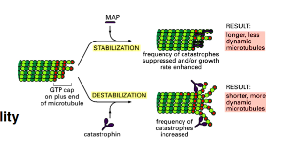
Microtubule-Associated Proteins (MAPs)
Note on terminology: MAP here stands for Microtubule-Associated Protein. This is different from the MAP (Mitogen-Activated Protein kinase) discussed in cell signaling. Context determines meaning.
Cells do not always want dynamically unstable microtubules. Many cellular functions require stable, persistent microtubules. A diverse set of proteins bind to microtubules and regulate their stability, organization, and dynamics. These are grouped functionally into four categories:

Capping / Nucleating Proteins
Capping / Nucleating Proteins
These proteins bind to the ends of microtubules and influence whether assembly or disassembly occurs. Some are stabilizing (nucleators), and some are destabilizing. An important example of a nucleating protein complex is gamma-TURC:
• Gamma-tubulin ring complex (gamma-TURC): A large ring-shaped complex composed of gamma-tubulin and several accessory proteins. It acts as a molecular template — a platform onto which alpha-beta tubulin dimers can assemble. By providing a pre-formed seed, gamma-TURC bypasses the slow nucleation step and dramatically shortens the lag phase of microtubule assembly. It caps and anchors the minus end, and nucleates growth from the plus end outward.
• Gamma-TURC is concentrated at the centrosome (microtubule organizing center, or MTOC), which is why the centrosome is the primary nucleation site for cytoplasmic microtubules in interphase cells.
• Plus end capping proteins can stabilize or destabilize the plus end depending on type.
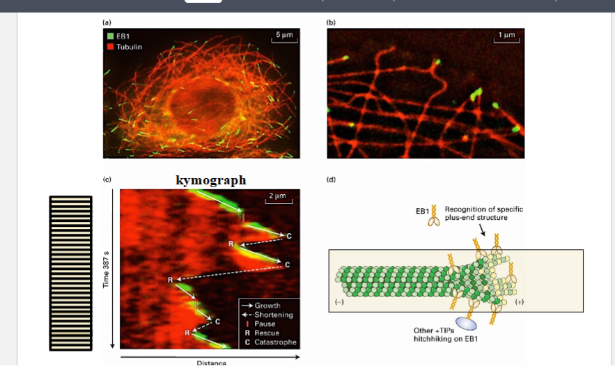
Destabilizing / Depolymerizing Proteins
Destabilizing / Depolymerizing Proteins
These proteins accelerate the loss of tubulin subunits from microtubules, either by promoting catastrophe at the ends or by physically cutting the microtubule.
Plus-End Tracking Proteins (+TIPs) — EB1 Example
A family of proteins called plus-end tracking proteins (or +TIPs) associate with the growing plus end of microtubules. An important and instructive example is EB1:
• When cells are imaged with fluorescently-labeled EB1, a green spot appears at the tip of each growing red (tubulin-labeled) microtubule. Early researchers saw EB1 at the tip of growing microtubules and concluded it must be stabilizing the plus end to allow growth.
• However, kymograph analysis revealed that EB1 is absent during microtubule shrinkage. Further work showed that EB1 actually destabilizes the plus end. It is this destabilizing action that triggers the catastrophe event seen in kymographs.
• EB1 appears at the growing end because it specifically recognizes the structural conformation of the GTP-tubulin at the tip of a growing microtubule. When it destabilizes that tip sufficiently, catastrophe occurs, EB1 dissociates, and the microtubule shrinks. When the microtubule is rescued and starts growing again, EB1 returns to the new plus end.
• Correction of textbook error: Some textbooks describe +TIPs as stabilizing the plus end. This is incorrect based on current experimental data — they are destabilizers that promote catastrophe.
Severing Proteins — Katanin
Katanin (named after the Japanese samurai sword "katana" by its discoverer, Dr. Ron Vale, who was fascinated by Japanese culture) is a protein that physically cuts microtubules along their length — not just at the ends.
• When katanin severs a microtubule in the middle, it generates two new ends. Each newly exposed internal end is composed of GDP-tubulin (since the internal lattice is GDP-tubulin). These unstable GDP-tubulin ends immediately begin depolymerizing rapidly.
• The result is rapid and complete disappearance of the microtubule — not just fragmentation into stable pieces. This is because cutting in the middle exposes GDP-tubulin at the new ends, which drives rapid depolymerization from both new ends simultaneously.
• Katanin therefore provides a rapid mechanism for completely eliminating a microtubule rather than waiting for it to depolymerize from its ends.
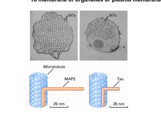
Cross-Linking Proteins
Cross-Linking Proteins
Cross-linking MAPs bind to the lateral surface (side) of microtubules and bridge them to other structures. They are important for organizing microtubule arrays and maintaining their spacing.
• MAP2: A large cross-linking protein found predominantly in neurons. Its length holds microtubules relatively far apart from each other (approximately 25 nm spacing visible in electron micrographs).
• Tau: A smaller cross-linking protein also found in neurons. Because it is shorter than MAP2, it holds microtubules closer together. Tau is clinically important — hyperphosphorylated, aggregated tau forms neurofibrillary tangles in Alzheimer's disease.
• Cross-linker length determines microtubule spacing: Longer cross-linkers → microtubules farther apart. Shorter cross-linkers → microtubules closer together. This can be directly observed in electron micrographs.
• Not all cross-linking is microtubule-to-microtubule: Some cross-linking proteins link microtubules to organelle membranes or to the plasma membrane, which is important for positioning organelles and for processes like mitosis.
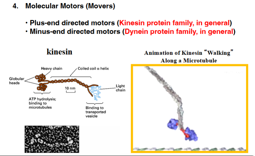
Molecular Motor Proteins
Molecular Motor ProteinsA. Why Motor Proteins Are Necessary
Large organelles and vesicles cannot simply diffuse to where they need to go within the cytoplasm. The cytoplasm is viscoelastic and has high macroviscosity — free diffusion is only possible for particles smaller than approximately 10 nm in diameter. Organelles are much larger than this. Furthermore, diffusion is a random process and cannot account for the highly directional, rapid movement of organelles observed in cells.
Motor proteins solve this problem. They physically link to organelles or vesicles and walk along microtubules (which serve as the cell's transportation highways), converting chemical energy from ATP hydrolysis into directional mechanical movement.
B. Two Major Classes of Microtubule-Based Motors
• Kinesins (plus-end directed, in general): Walk toward the plus end of microtubules. Because plus ends generally point toward the cell periphery (in most cell types), kinesins typically carry cargo away from the cell center — toward the plasma membrane, axon terminus, or cilium tip.
• Dyneins (minus-end directed, in general): Walk toward the minus end of microtubules. Because minus ends point toward the centrosome/cell center in most cells, dyneins carry cargo toward the cell center — toward the nucleus, or back toward the cell body in an axon.
Important qualifier: The "in general" caveat is significant. Some kinesins walk toward the minus end, and some dyneins have modified directionality. Direction of movement must be confirmed experimentally for each specific motor protein.
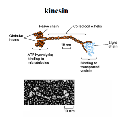
Structure of Kinesin
Structure of Kinesin
The conventional kinesin molecule (kinesin-1) has the following architecture:
• Two heavy chains: The major structural component. Each heavy chain is a large polypeptide. The two heavy chains wrap around each other in a coiled-coil alpha-helix along most of their length, forming a long stalk.
• Globular head domains: At one end of each heavy chain is a large globular motor domain (the "head"). These heads are where ATP hydrolysis occurs and where microtubule binding takes place. The two heads alternate in their binding to the microtubule, producing a hand-over-hand walking motion — interpreted as kinesin "walking" along the microtubule.
• Light chains: At the opposite end of the heavy chain stalk, smaller kinesin light chain polypeptides associate with the heavy chains. The light chains are the cargo-binding region — they physically connect kinesin to the organelle or vesicle that is being transported. The light chain is the link between the motor and its cargo; the walking machinery is in the heads.
Kinesin: Structure and Mechanism
Walking Mechanism
• Kinesin moves in steps of 16 nanometers per step along the microtubule.
• One head group is always bound to a beta-polypeptide of tubulin on the microtubule at any given time.
• When ATP binds to the forward head group, it triggers a conformational change in the neck region of the molecule.
• This conformational change causes the trailing head group to swing forward and land on the next beta-tubulin subunit.
• The ATP that was bound hydrolyzes to ADP, ADP is released, and a new ATP binds — and the cycle repeats.
• There is always at least one head group attached to the microtubule at all times. This is essential for efficient cargo transport — losing contact with the substrate would make movement ineffective, just as a person carrying a heavy object must always have at least one foot on the ground.
Speed and Processivity
Kinesin moves at approximately 1 to 2 micrometers per second. To put this in biological context, an E. coli-like cell that is 4 micrometers in diameter could be traversed by a kinesin molecule in just 4 seconds.
The ability of kinesin to stay in continuous contact with its substrate — traveling up to a full micrometer without detaching — is called processivity. Kinesin and dynein are both described as processive molecules. DNA polymerase is another well-known example of a processive enzyme, as it moves continuously along a single strand of DNA during replication without detaching.
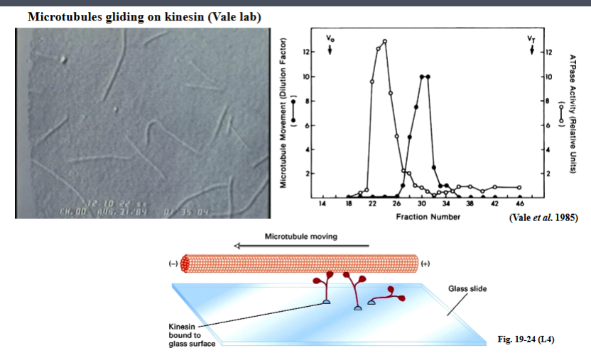
The Squid Axoplasm Model and Discovery of Kinesin
The story of kinesin's discovery is a landmark in cell biology. Dynein, which moves toward the minus end of microtubules, was discovered first. The challenge was finding the motor responsible for moving cargo toward the plus end of microtubules — the mystery motor protein that would come to be known as kinesin.
The Squid Axon Model System
This research was conducted at the Marine Biological Laboratory at Woods Hole on Cape Cod. The organism of choice was the squid, favored by neurobiologists because squid have exceptionally large neurons — visible to the naked eye — including a giant axon. Researchers could take a single neuron, place it on a microscope slide, and observe movement inside the axon directly.
To study axonal contents, researchers used safety scissors to cut the end of a neuron and allowed the contents to spill out, or used a small roller to squeeze out the cytoplasm from the axon. The cytoplasm of an axon is specifically called axoplasm. When this axoplasm was examined under a microscope, organelles could be seen moving in both directions along microtubules.
In an axon, all microtubules are oriented in parallel arrays with their plus ends pointing toward the end of the axon. Organelles moving back toward the cell body (toward the minus end) were attributed to dynein. The mystery was: what motor was moving organelles toward the plus end, toward the axon terminus?
The Problem with the Old Approach
The initial strategy was to use the same biochemical fractionation protocols developed to isolate dynein — looking for fractions with peak ATPase activity. Since dynein is known to consume large amounts of ATP, finding a high-ATPase fraction seemed like a logical starting point. Multiple labs pursued this approach, working in secrecy. No one found the mystery protein.
The reason the approach failed: the same biochemical protocols used to isolate dynein were destroying the ATPase activity of kinesin. The mystery protein's enzymatic activity was being eliminated unintentionally during fractionation, so it was invisible to the standard assay.
Vale's Breakthrough: The In Vitro Microtubule Gliding Assay
Ron Vale's key insight was to think differently. Instead of looking for the protein moving along a microtubule, he flipped the question: look for the microtubule moving.
Vale assembled stabilized microtubules (so they could not depolymerize) and then coated a glass slide with a drop of each axoplasm fraction. He then placed microtubules on top of the coated slide and asked: do the microtubules move?
Since kinesin is a plus-end directed motor, and the motor was immobilized on the glass slide, the microtubule would be pushed in the direction of its minus end. This is because as the motor walks toward the plus end of the microtubule, the microtubule itself moves in the opposite direction — toward its minus end.
Key Data from Vale's Paper
Vale's chromatographic fractionation results showed that the peak of microtubule movement activity (solid black dots) was located around fraction 32. Meanwhile, the peak of ATPase activity (open circles) was at fraction 24 — a completely different fraction. This explained why the old approach had failed: most of kinesin's ATPase activity had been destroyed during fractionation, so it wasn't showing up where researchers expected.
The in vitro gliding assay was extremely sensitive because even a single kinesin molecule can move an entire microtubule. Even if 99.99% of kinesin molecules had been destroyed, the remaining few were enough to power microtubule movement — something standard bulk ATPase measurements would completely miss.
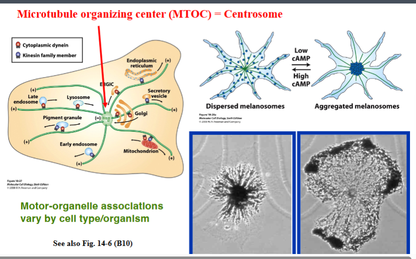
Organelle Transport and the Centrosome
Organelle Transport and the Centrosome
The polarized microtubule array and the two classes of motor proteins together form a directed transport system. Kinesins drive cargo toward plus ends (generally outward), while dyneins drive cargo toward minus ends (generally inward toward the centrosome). Different organelles associate with specific motor proteins, and this association can be regulated by signaling pathways.
Example — melanosomes: In pigment cells, melanosomes (pigment-containing organelles) can be rapidly redistributed between the cell center and the periphery in response to hormonal signals that change cAMP levels. High cAMP: melanosomes disperse outward (kinesin-driven). Low cAMP: melanosomes aggregate toward the centrosome (dynein-driven). This is a visually striking example of regulated bidirectional transport.
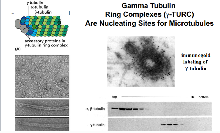
The Centrosome as MTOC
The Centrosome as MTOC
The centrosome is the primary microtubule organizing center (MTOC) in animal cells. It contains:
• A pair of centrioles: Cylindrical structures made of triplet microtubules arranged in a 9-fold symmetric pattern.
• Pericentriolar material (PCM): An amorphous cloud of protein surrounding the centrioles. The PCM contains gamma-TURC complexes, which are the actual nucleating sites for microtubule assembly.
Microtubules grow outward from the centrosome with their minus ends anchored at the gamma-TURC and their plus ends extending into the cytoplasm. This organization creates the classic "aster" pattern seen in both interphase cells and in cells preparing for mitosis.
Gamma-tubulin was discovered by Dr. Bill Oakley at Ohio State University through genetic analysis of fungi. He identified a protein highly homologous in sequence to alpha- and beta-tubulin and named it gamma-tubulin. Gamma-tubulin and its associated accessory proteins in the gamma-TURC complex form a template onto which alpha/beta-tubulin heterodimers bind, initiating microtubule nucleation. Because this pre-formed platform exists, there is very little lag time before rapid microtubule assembly begins.
The location of gamma-tubulin within the centrosome was determined using immunogold labeling — a technique analogous to indirect immunofluorescence microscopy, but adapted for electron microscopy. Instead of a fluorescent tag on the secondary antibody, a gold particle is used. Gold particles appear as small black dots in electron micrographs because they deflect electron beams. Results showed gold particles concentrated in the pericentriolar material — not at the centrioles themselves — confirming that gamma-tubulin (and thus microtubule nucleation) occurs in the PCM.
Prokaryotes Have Cytoskeletons Too
Prokaryotes Have Cytoskeletons Too
For decades, it was assumed that cytoskeletons were an exclusively eukaryotic feature. This assumption has been overturned. It is now established that prokaryotes — bacteria and archaea — also possess cytoskeletal elements, though they are structurally and compositionally distinct from eukaryotic cytoskeletal proteins.
• Asgard archaea: A recently characterized phylum of archaea that appears to harbor proteins capable of forming polymer structures that resemble eukaryotic microtubules. These form smaller-diameter polymer rings and have structural similarities to alpha-beta tubulin, though fewer protofilaments. This finding is significant because Asgard archaea are thought to be among the closest prokaryotic relatives of eukaryotes, and may illuminate the evolutionary origin of the microtubule cytoskeleton.
• FtsZ (in bacteria): A protein that forms a heterodimer and polymerizes into ring-like filamentous structures at the site of cell division in bacteria. FtsZ is a GTPase that assembles and disassembles much like tubulin. Its three-dimensional structure is remarkably similar to alpha-beta tubulin even though the primary amino acid sequence is quite different. FtsZ is considered the evolutionary ancestor of eukaryotic tubulin — an example of divergent evolution where sequence has changed but structural fold has been conserved.
• Other prokaryotic cytoskeletal proteins include MreB (an actin homolog important for maintaining rod cell shape in bacteria), crescentin (an intermediate filament-like protein in Caulobacter), and various other filament-forming proteins discovered across the bacterial domain.
Key evolutionary insight: The same higher-order polymer structures and functions (cell shape maintenance, cell division, etc.) can be achieved by proteins with very different primary sequences, provided the three-dimensional protein fold and polymerization properties are conserved. Structure and function are more evolutionarily conserved than sequence.
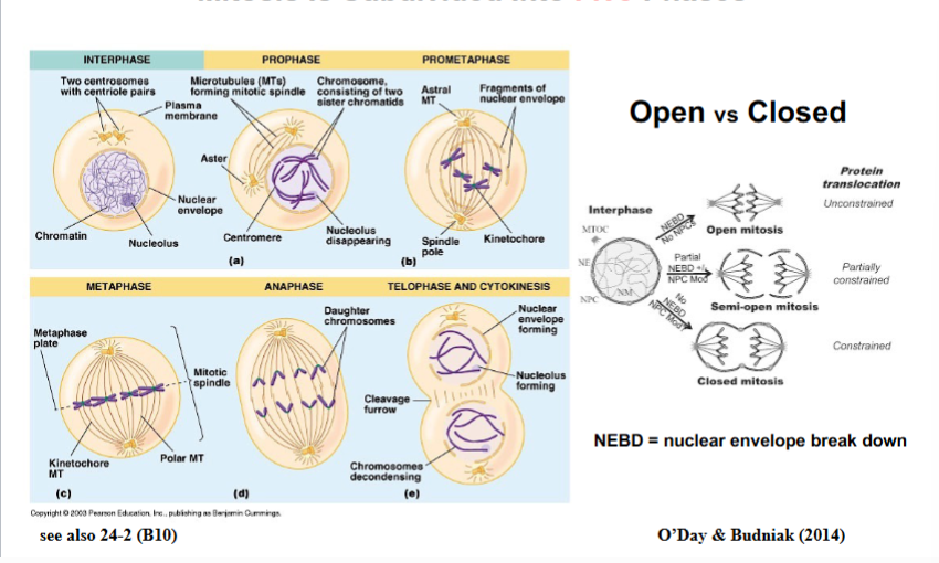
Mitosis and the Role of Motor Proteins
Mitosis and the Role of Motor Proteins
Mitosis is divided into five phases: prophase, prometaphase, metaphase, anaphase, and telophase. Cytokinesis (division of the cytoplasm) may be listed alongside telophase depending on the textbook. When a cell is not undergoing mitosis, it is in interphase.
NEBD= nuclear envelope break down
In animal cells (and human cells), mitosis is open — meaning the nuclear envelope breaks down during the process and is reassembled at the end. In some organisms such as fungi, mitosis is closed — the nuclear envelope remains intact throughout, and the entire mitotic process occurs within the nucleus. During closed mitosis, nuclear pore complexes become nonspecific, allowing relatively free movement of molecules in and out of the nucleus.
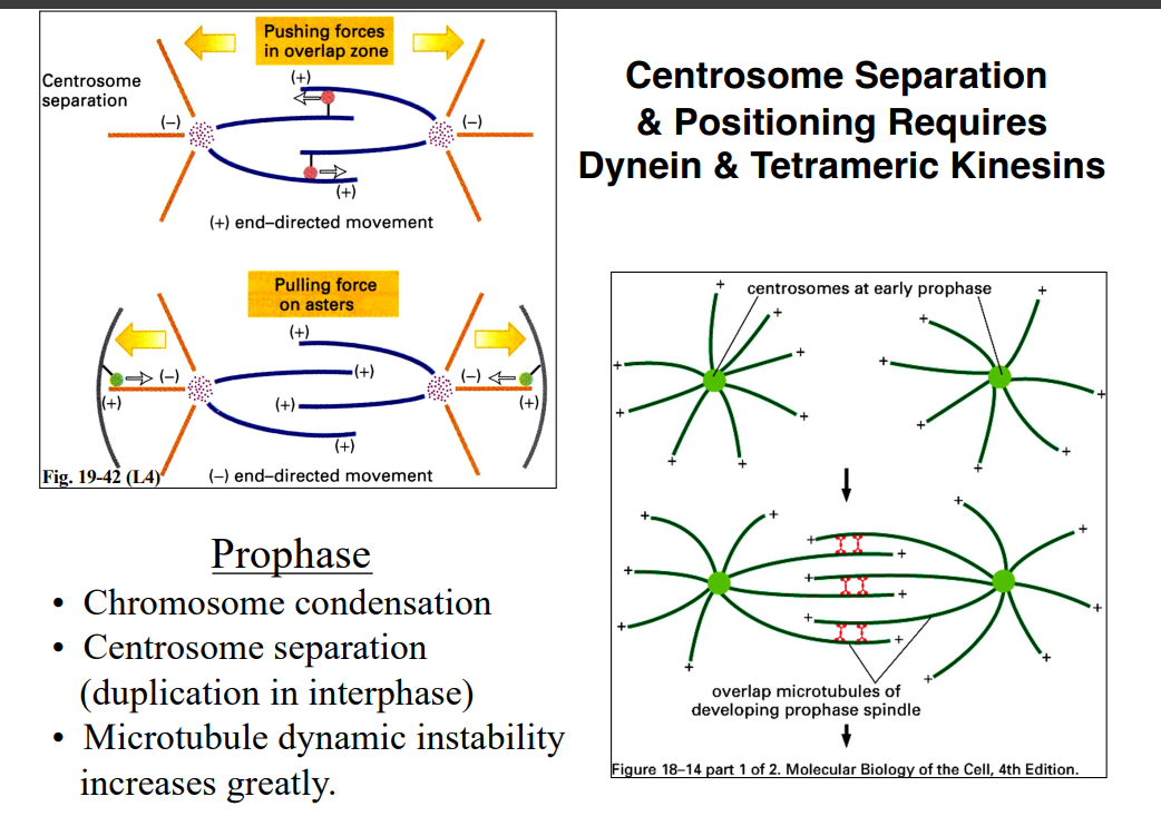
Prophase
Prophase
• Chromosome condensation: Chromosomes in their territories begin compacting. Condensed chromosomes are far more efficiently moved than loose chromatin (described as being like trying to move balls of spaghetti).
• Centrosome separation: The cell enters prophase with two centrosomes (duplicated during interphase). These two MTOCs move to opposite poles of the cell through the action of motor proteins. Two types of forces are involved:
◦ Pushing force: Microtubules from the two centrosomes interdigitate (overlap) at their plus ends. A tetrameric kinesin (two kinesin molecules bound tail-to-tail) bridges the two microtubules with head groups on each. As these head groups walk toward the plus ends of each microtubule, the microtubules slide past each other, pushing the centrosomes apart.
◦ Pulling force: Astral microtubules (extending from the centrosomes to the cell cortex) interact with dynein anchored at the plasma membrane. Dynein walks toward the minus end of these microtubules, effectively pulling each centrosome toward the plasma membrane.
• Increased microtubule dynamic instability: Stabilizing MAPs that normally keep microtubules stable are no longer associated with the microtubules during mitosis, causing microtubules to grow and shrink much more rapidly.
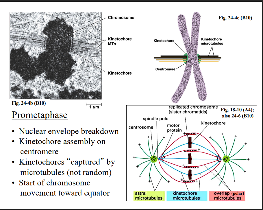
Prometaphase
Prometaphase
• Nuclear envelope breakdown: The nuclear lamina — a network of lamin polymer fibers — disassembles. This destabilizes the nuclear envelope membrane, causing it to fragment into smaller pieces.
• Kinetochore assembly on centromere: A kinetochore is a massive multi-protein complex that assembles at the centromere — a specific region of DNA at the middle of each chromosome.
◦ In simple cells: centromeres may be 40 to 100 kilobases in size; one microtubule attaches per kinetochore
◦ In mammalian cells: centromeres with unique DNA sequences can be up to 2 megabases in size; dozens of microtubules attach per kinetochore
• Microtubule capture of chromosomes: Because microtubules are highly dynamic during this phase (growing and shrinking rapidly), their capture of chromosomes at the kinetochore appears to be a random process but its not. As a growing microtubule contacts the kinetochore of a condensed chromosome, it captures the chromosome. Once captured, motor proteins begin moving the chromosome toward the center of the cell — a process called congression.
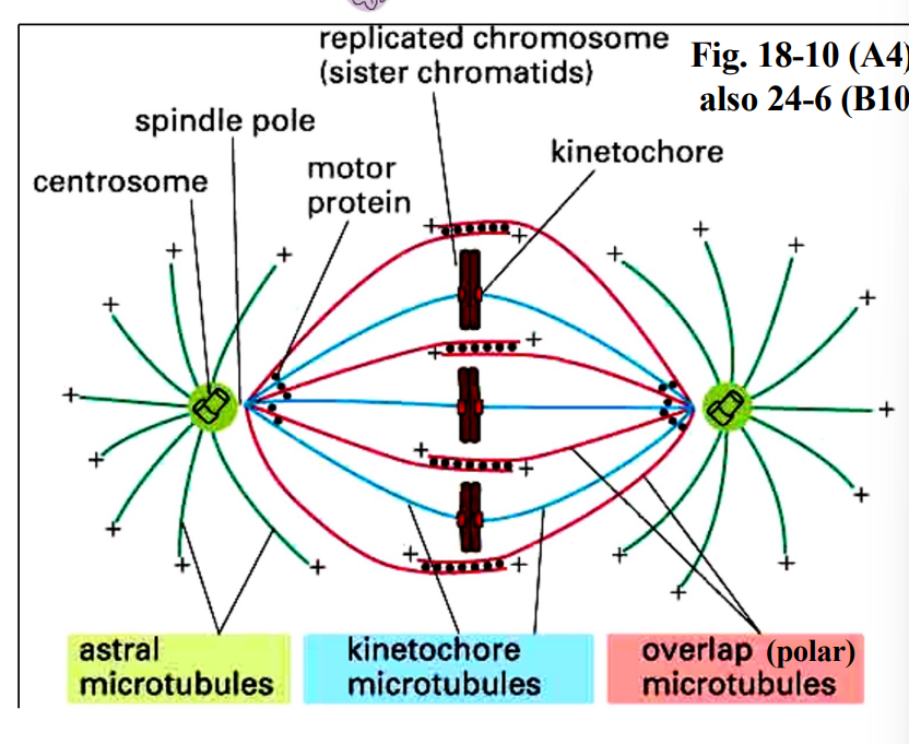
Prometaphase
The Mitotic Spindle and Microtubule Types
During prometaphase, the two centrosomes that were duplicated during interphase and separated during prophase have taken up positions on opposite sides of the cell, establishing the poles of the mitotic spindle. The motor proteins responsible for this separation are dynein and tetrameric kinesins, which slide microtubule arrays of the two centrosomes past each other, pushing the centrosomes apart. Once positioned, these centrosomes are referred to as spindle pole bodies.
Radiating from each centrosome are three functionally distinct types of microtubules:
• Kinetochore microtubules — these extend from the centrosome and make direct contact with the kinetochore, a protein structure assembled on the centromere region of each chromosome. These are the microtubules responsible for physically moving chromosomes.
• Polar (overlap) microtubules — these extend from the centrosome but do not contact chromosomes. Instead, they interact with polar microtubules emanating from the opposite centrosome, overlapping in the middle of the cell. These are critical for pushing the poles apart during anaphase B.
• Astral microtubules — these extend outward from the centrosome toward the plasma membrane (cell cortex). They help position and stabilize the spindle within the cell.
Together, the two spindle pole bodies plus all three categories of radiating microtubules form the structure called the mitotic spindle.
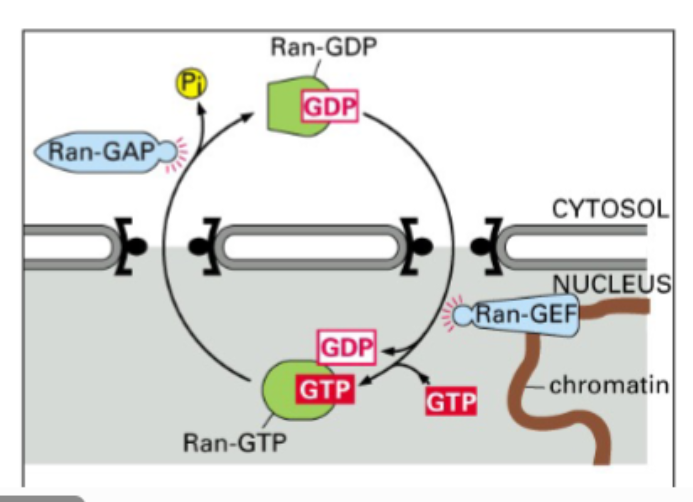
Spindle Formation in Acentrosomal Cells (Higher Plants)
In cells that lack centrosomes, such as those found in higher plants, a mitotic spindle is still formed through a chromatin-based mechanism. The chromatin itself has an associated protein called a RanGEF (a nucleotide exchange factor for the Ran GTPase). This RanGEF promotes the conversion of Ran-GDP to Ran-GTP in the vicinity of the chromatin.
Ran-GTP, the active form, causes the release of microtubule-stabilizing factors that are otherwise sequestered by importin. Once free of importin, these stabilizing factors promote microtubule formation. The microtubules then self-organize — aided by motor proteins — into a bipolar array that resembles a conventional mitotic spindle. This has been demonstrated experimentally by coating plastic beads with random pieces of chromatin and placing them in a cell extract, where microtubules form around the beads and organize into a bipolar spindle.
This process parallels how Ran-GTP functions in nuclear import, where it releases cargo from importin. The same molecule uses the same molecular logic but in a different cellular context.
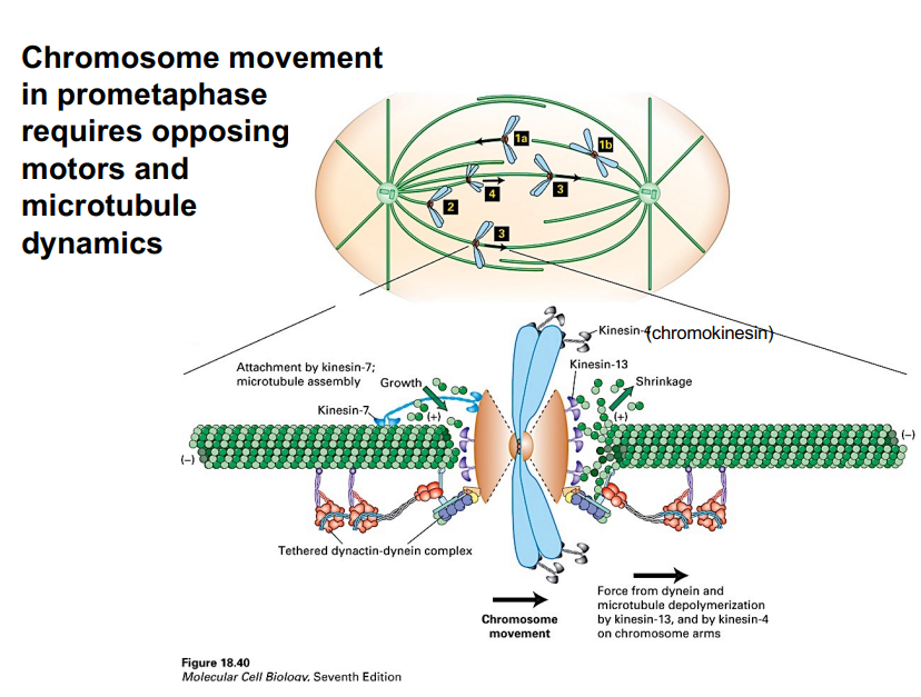
Chromosome Movement to the Metaphase Plate
Chromosome Movement to the Metaphase Plate
During prometaphase, chromosomes must move from wherever they are within the cell to the midline (the metaphase plate) at the center. This movement is driven by opposing forces generated by multiple motor proteins and microtubule dynamics acting simultaneously.
Looking at a sister chromatid pair, several forces are acting at once:
• On the side where the kinetochore microtubule is growing, a kinesin (kinesin-7) walks toward the plus end of the microtubule. Because it is attached to the chromosome, this walking action pushes the chromosome pair toward the center of the cell.
• On the opposite side, another microtubule is being shortened by a different kinesin acting as a depolymerizer rather than a traditional motor. This is kinesin-13, which does not walk along microtubules in a directional sense but instead destabilizes the microtubule, causing it to shrink.
• Dynein, a minus-end-directed motor protein, is also associated with the kinetochore and the microtubule on this side. As kinesin-13 depolymerizes the microtubule, dynein walks toward the minus end and pulls the chromosome toward that pole.
An additional force contributes to chromosome movement: chromokinesin (kinesin-4) binds to the arms of the chromosomes and connects them to polar microtubules. As chromokinesin walks toward the plus end of the polar microtubule, it pulls the chromosome arms forward. For many years, this apparent forward bending of chromosome arms was attributed to a hypothetical 'polar ejection force' thought to emanate directly from the pole — but no such force exists. The chromosome arms are being actively pulled, not pushed.
It is more important to understand the location and function of these motor proteins than to memorize their specific numerical designations. The one name worth knowing is chromokinesin, the kinesin associated with the chromosome arms.
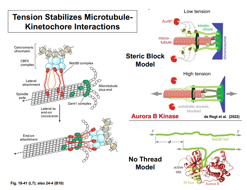
Stable Kinetochore-Microtubule Attachment
Stable Kinetochore-Microtubule Attachment
When a microtubule first makes contact with a kinetochore, the initial interaction is weak. This typically occurs when the microtubule grazes the kinetochore laterally (a 'glancing blow') rather than making direct end-on contact. The kinetochore is organized into two layers — an inner layer and an outer layer — and the key complex in the outer kinetochore layer responsible for connecting to microtubules is the NDC80 complex (also written as Ndc80). This is an important protein complex to know.
The lateral attachment mediated by NDC80 is initially weak. Over time, the geometry must rearrange so that the end of the microtubule makes direct contact with the kinetochore, creating an end-on attachment. Once this end-on attachment is established, tension from the various motor forces causes the interaction to strengthen.
The molecular mechanism by which tension strengthens the attachment involves a kinase called Aurora B kinase — another important name to know. Aurora B kinase phosphorylates the NDC80 complex. When NDC80 is heavily phosphorylated, its interaction with the microtubule is weak. This is because phosphorylation adds many negatively charged phosphate groups to the NDC80 proteins, and the surface of a microtubule also carries a net negative charge due to exposed acidic amino acids. Like charges repel, so a highly phosphorylated NDC80 is electrostatically repelled from the microtubule.
Two models have been proposed to explain how tension reduces Aurora B kinase activity and thereby strengthens the attachment:
• Steric Block Model — tension physically rearranges the outer kinetochore complex so that Aurora B kinase can no longer access the NDC80 proteins that are its phosphorylation substrates. The structural change sterically blocks the kinase.
• No Thread Model — tension stretches the NDC80 proteins so extensively that they cannot be threaded into the active site of Aurora B kinase, preventing phosphorylation from occurring efficiently.
Both models converge on the same functional outcome: reduced phosphorylation of NDC80 produces a tight, stable kinetochore-microtubule interaction. The exact mechanism remains under investigation.
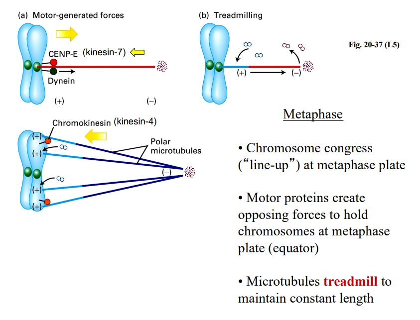
Metaphase
Metaphase
At metaphase, all chromosomes have aligned at the metaphase plate — the midline of the cell. This alignment is the result of all the opposing motor forces reaching a state of balance. The kinetochore microtubules from both poles are exerting forces in opposite directions, and when these forces are equal, each chromosome is held stably at the center.
During this phase, the kinetochore microtubules maintain a constant length. This does not mean they are static — in fact, they are highly dynamic. What is happening is a process called treadmilling: tubulin subunits are being added at the plus end (near the kinetochore) at the same rate they are being lost at the minus end (near the spindle pole). The net result is a microtubule of constant length where individual subunits are continuously moving from one end to the other.
Treadmilling is actually quite rare for microtubules — it is a much more common behavior for microfilaments (actin filaments). Its occurrence in metaphase kinetochore microtubules is a notable exception. A practical consequence of treadmilling is that a tubulin subunit added at the plus end will gradually travel along the microtubule and eventually be released at the minus end.
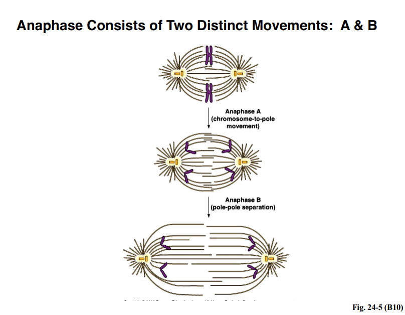
Anaphase
Anaphase
Anaphase is divided into two mechanistically distinct sub-phases: Anaphase A and Anaphase B.
A. Anaphase A — Chromosome-to-Pole Movement
In Anaphase A, the sister chromatids separate and each chromatid moves toward its respective spindle pole. The primary mechanism is the shortening of kinetochore microtubules. Kinesins acting as depolymerizers cause the microtubule to shrink from both the plus end (at the kinetochore) and the minus end (at the spindle pole). As the kinetochore microtubule shortens, the chromosome is pulled along with it toward the pole.
Additionally, dynein anchored at the astral microtubules pulls on the spindle pole itself, maintaining tension across the entire spindle structure and contributing to the movement of chromosomes toward the poles.
B. Anaphase B — Pole-to-Pole Separation (Spindle Elongation)
In Anaphase B, the spindle poles themselves move apart from each other, increasing the overall length of the cell in preparation for division. This is driven by tetrameric kinesins (four-headed kinesins) that crosslink the overlapping polar microtubules from opposite poles. Each kinesin molecule walks toward the plus end of the polar microtubule it is bound to, and since the polar microtubules from the two poles are interdigitated in antiparallel orientation, the two arrays slide past each other. This sliding force pushes the two poles farther apart.
As the poles move apart, the polar microtubules would otherwise run out of overlap. To prevent this and to keep the poles moving farther apart, the cell simultaneously allows tubulin polymerization at the plus ends of the polar microtubules. The microtubules grow longer as the poles separate, providing more track for the tetrameric kinesins to continue walking. This coordinated growth and sliding produces spindle elongation.
This is the same mechanism used during prophase to initially separate the centrosomes — the same tetrameric kinesins on overlapping microtubules.
Telophase (Brief Overview)
Telophase involves the reconstruction of the nucleus in each daughter cell. The nuclear envelope, which was fragmented into small vesicles during mitosis, is reassembled around each set of chromosomes. The nuclear lamina, a meshwork of intermediate filaments just inside the nuclear envelope, is also reformed to stabilize the newly reconstituted envelope. Various nuclear compartments and neighborhoods characteristic of an interphase nucleus are re-established as chromosomes begin to decondense.
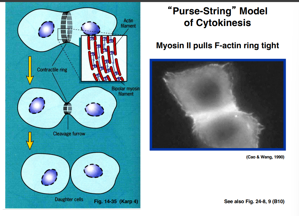
Cytokinesis
CytokinesisA. The Purse-String Model
Following mitosis, the cell must physically divide its cytoplasm into two separate daughter cells through a process called cytokinesis. Unlike mitosis, cytokinesis does not rely on microtubules — it relies on the microfilament (actin) cytoskeleton.
The mechanism is described by the purse-string model. A ring of microfilaments assembles just beneath the plasma membrane at what will become the division plane. This structure is called the contractile ring. The contractile ring is composed of actin microfilaments, and it is attached to the inner surface of the plasma membrane around the full circumference of the cell.
As the microfilaments in the contractile ring slide past each other — driven by the motor protein myosin — the ring constricts. This constriction creates an indentation in the cell surface called the cleavage furrow. The furrow deepens as the ring tightens, much like pulling the drawstring of a purse. Eventually the constriction reaches the point of scission, and the two daughter cells are completely separated.
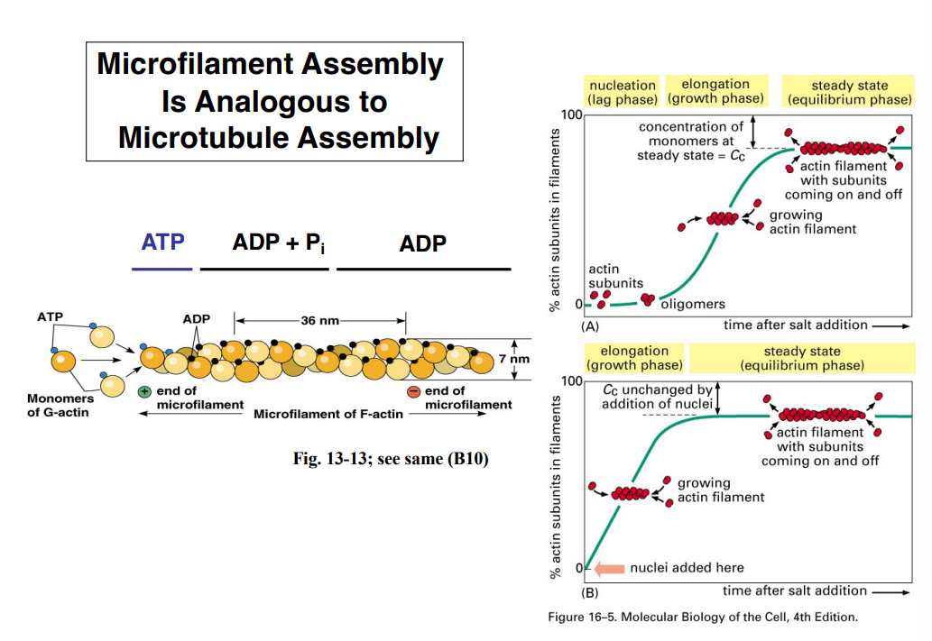
Microfilaments — Structure and Assembly
Microfilaments — Structure and AssemblyA. Polarity and Nomenclature
Microfilaments are cytoskeletal polymers composed of a subunit protein called actin. Like microtubules, microfilaments are polarized — they have a structurally and functionally distinct plus end and minus end. However, the terminology used for microfilaments differs from that used for microtubules:
• The plus end of a microfilament is called the barbed end.
• The minus end is called the pointed end.
This nomenclature arose from a classic experimental observation. When myosin head domains are purified (by enzymatically cleaving myosin heavy chains with a protease to release the globular head fragments) and then mixed with microfilaments, the head domains bind along the length of the filament. Under electron microscopy, the bound heads give the filament a chevron-like, arrowhead appearance. The tip of the arrowhead points toward the minus (pointed) end, and the wider base of the arrowhead is at the plus (barbed) end.
B. Actin Monomers (G-actin) and the Nucleotide
Actin monomers are called G-actin (globular actin). Unlike tubulin, which is a heterodimer of alpha and beta subunits, actin is a monomer — a single polypeptide chain. Each G-actin monomer binds a single ATP molecule in a central cleft within the protein.
When actin monomers assemble into filaments, the polymer is called F-actin (filamentous actin). This is what is commonly referred to as a microfilament. The assembly process is analogous to microtubule assembly: as filaments grow, the ATP within actin subunits is hydrolyzed. Subunits that have recently joined still carry ATP; those that joined earlier are in an ADP+Pi state (phosphate still bound); and the oldest subunits have released the inorganic phosphate and carry only ADP. This gradient of nucleotide states along the filament has important consequences for filament dynamics.
C. Critical Concentration and Assembly Kinetics
Like microtubules, microfilaments assemble from monomers only when the monomer concentration exceeds the critical concentration. Below the critical concentration, the polymer does not grow — any existing polymer will disassemble. The critical concentration for actin assembly is approximately 0.1 micromolar, which is about 100-fold lower than the critical concentration for microtubule assembly (approximately 10 micromolar).
The kinetics of actin assembly follow the same general pattern as microtubule assembly: there is a lag phase (nucleation), followed by rapid growth (elongation), and finally a steady state (equilibrium phase). Adding a nucleator protein eliminates the lag phase by providing pre-formed oligomers that serve as seeds for filament growth. Critically, nucleators do not change the critical concentration — the plateau level of assembled subunits at steady state remains the same whether a nucleator is present or not.
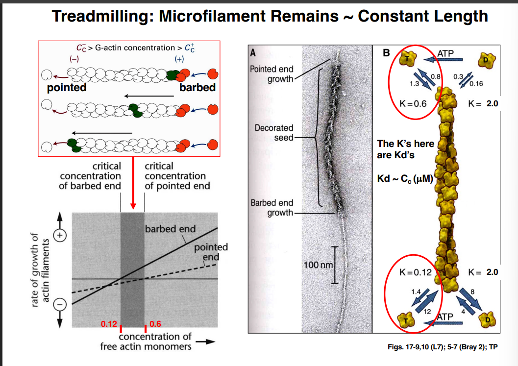
Microfilament Treadmilling
Microfilament Treadmilling
Treadmilling is the phenomenon where a polymer maintains a constant overall length while individual subunits continuously add at one end and fall off at the other. For microfilaments, treadmilling is very common — in contrast to microtubules, where treadmilling is rare (with the notable exception of metaphase kinetochore microtubules, as described above).
The basis for treadmilling lies in the fact that the two ends of a microfilament have different critical concentrations:
• The barbed end (plus end) has a lower critical concentration of approximately 0.12 micromolar — meaning assembly occurs there at relatively low actin concentrations.
• The pointed end (minus end) has a higher critical concentration of approximately 0.6 micromolar — meaning assembly at this end requires a higher concentration of free monomers.
This difference in critical concentrations creates three distinct concentration zones:
• Below 0.12 micromolar: neither end grows; both ends disassemble.
• Between 0.12 and 0.6 micromolar (the treadmilling zone): the barbed end grows (net addition of subunits) while the pointed end disassembles (net loss of subunits). The filament maintains a roughly constant length, but individual subunits move through the polymer from barbed to pointed end over time.
• Above 0.6 micromolar: both ends grow simultaneously.
Tom Pollard, a researcher who was long at Yale University and more recently at UC Berkeley, contributed significantly to working out the detailed rate constants for actin assembly and disassembly at each end. These rate constants allow calculation of the dissociation constant (Kd) for each end, which approximates the critical concentration.
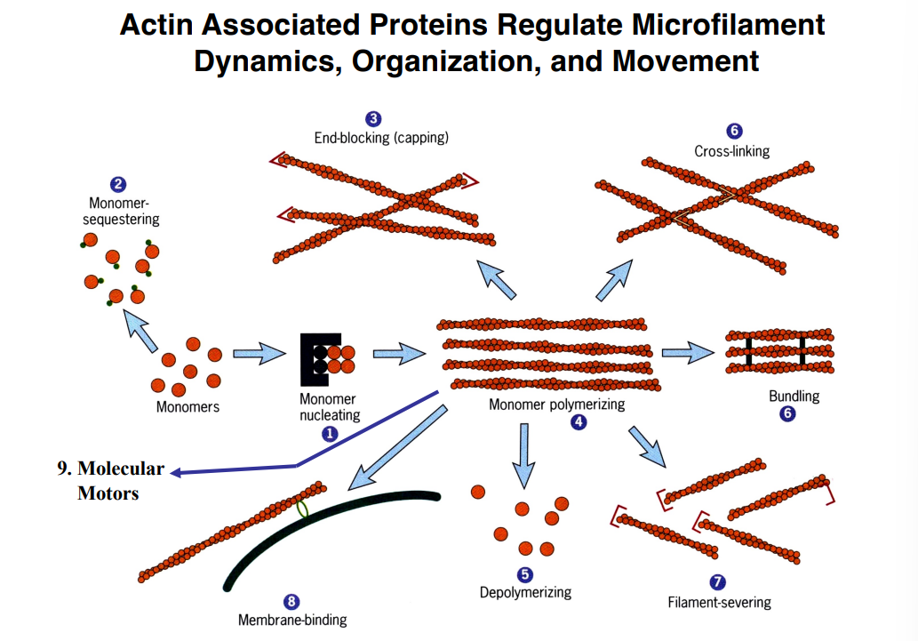
Actin-Associated Proteins
Actin-Associated Proteins
Microfilaments interact with a large number of accessory proteins that regulate their dynamics, organization, and interactions with other cellular structures. The major categories of actin-associated proteins include:
• Nucleators — promote the formation of new filaments by providing a seed or template, eliminating the lag phase of assembly without affecting critical concentration.
• Monomer-sequestering proteins — bind free G-actin monomers and hold them in a pool unavailable for polymerization. By regulating the size of this free pool, the cell can rapidly switch between filament growth and shrinkage.
• Depolymerizing proteins — promote disassembly of existing filaments.
• Severing proteins — cut existing filaments, creating new free ends.
• Capping proteins — bind to the ends of filaments and prevent further addition or loss of subunits.
• Cross-linking proteins — connect multiple filaments into networks.
• Bundling proteins — organize filaments into tight parallel bundles.
• Membrane-binding proteins — anchor microfilaments to the plasma membrane.
Myosin is the primary motor protein associated with microfilaments and will be covered in detail in the next lecture.