Macroeconomics

How is the dynamic IS curve derived?

• Consumption and investment functions are substituted into the GDP identity

• Y^D = C + I + G = c₀ + c₁(1 - t)y + a₀ - a₁r + G

• Impose the equilibrium condition, output = expenditure

• y = 1/(1 - c₁(1 - t)) (c₀ + a₀ + G - a₁r) = k(c₀ + a₀ + G) + ka₁r = A - ar

• This represents goods market equilibrium (demand = supply)

What does A - ar describe?

• This describes output as a multiple of exogenous spending decisions, adjusted for the negative effect of higher interest rates on investment

The slope and constants of the IS curve

• y = A - ar, where the inverse relationship between output and investment can be plotted in r-y space, r = A/a - (1/a)y

• a = ka₁, where k is the multiplier, where 0 < k < 1, 0 < t < 1, and real interest elasticity of investment a₁ > 0 (how much investment changes w.r.t real interest rate)

• Thus a > 0, so in the IS curve where -ar exists, the slope is negative

• The exogenous component, A = k(c₀ + a₀ + G) involves (via k) the MPC, the marginal tax rate, autonomous consumption, autonomous investment, and government spending

What are the three expenditure components?

• c = 𝑐₀ + 𝑐₁(1 − 𝑡)𝑦 is Real consumer spending, whose equation makes clear is assumed to not depend on 𝑟

• 𝐼 = 𝑎₀ −𝑎₁𝑟 is Real business investment, which depends on 𝑟

• 𝐺 is Government consumption/spending, which is assumed to not depend on r

What are properties of the IS curve?

• Downwards sloping meaning that high r means low y and low r means high y

• A higher multiplier means that the slope becomes flatter and vice versa (the multiplier, 1/(1-c₁(1-t)) increases via lower t or higher c₁)

• An increase in investment sensitivity to interest rates, a₁, flattens the slope

What shifts the IS curve?

• Any change in its exogenous components, c₀, a₀ or G

• The change in income resulting from these expenditure changes is given by the change in spending multiplied by the multiplier

Lag in the IS curve and the monetary policy transmission mechanism

• Typically, the curve avoids time-specific subscript to emphasise the general formula, but the dynamic curve is written as y_t = A - ar_{t - 1}

• CB sets an interest rate which is mediated through financial markets, affecting things like the exchange rate and asset prices before reaching the real economy in the labour market and in domestic prices

Properties of the Phillips Curve

• The output gap is negatively related to unemployment

• There is a positive relation between inflation and the output gap

• Downwards-sloping in π-u space, upwards-sloping in π-r space

Properties of wage-setting curve

• In equilibrium the market normally doesn’t clear, resulting in some unemployment because firms pay efficiency wages above a worker’s reservation wage to induce them to work hard

• At high levels of unemployment, a low wage is needed, and vice versa

• A positive output gap (rise in output) reduces unemployment, reducing cost of job loss therefore requiring higher wages

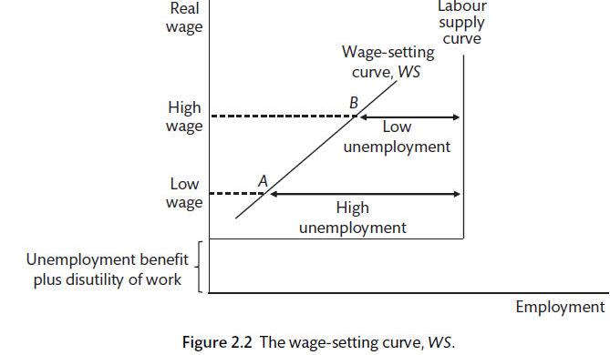
Supply shocks in the closed economy model

• These are only caused by shifts in the wage-setting or price-setting curves; understanding the models which motivate the Phillips curve are therefore crucial

Writing the Wage-setting curve

• w^WS = W/p^E = f(N, z_W), where z_W captures all the factors that might influence wage-pushes besides the natural rate of employment (like union power, increased bargaining etc)

• w^WS = W/p^E = α(y_t - y_e) + z_W is another way of writing it, because wages and inflation are positively correlated

• B is included in z_W, where B is a constant which represents the pecuniary and non-pecuniary benefits of not working including disutility from work (unemployment benefits)

What shifts the wage-setting curve down (supply shock)?

• Fall in unemployment benefits (amount, duration, increase in application difficulty or tougher eligibility criteria)

• Improvement in working conditions (reduction in net disutility of work)

• More/cheaper monitoring of work effort; lower cost of firing shirkers

• Unions have less bargaining power or legal protection leading to less union nominal markup

• These allow for higher costs of unemployment and lower efficiency wages to be paid

Wage inflation in the WS curve

• Taking logs of W/p^E = α(y_t - y_e) + z_W, derive (ΔW/W)_t = (ΔP^E/P^E)_{t - 1} + α(y_t - y_e)

  • Expected wage inflation is equal to expected inflation + economic activity pressures, assuming P^E = P_{t - 1}

• Therefore, the higher expected inflation is, the higher nominal wage growth will be

Properties of the price-setting curve

• Price changes depend positively on wage increases, negatively on productivity decreases, and assuming markup is fixed, not on the market

Writing the Price-Setting curve

• Prices depend on marginal costs, which is the nominal wage per unit of output, W/λ, as well as the markup, μ, which measures the extent to which prices exceed unit labour costs in percentage points

  • Very simple production function; labour is the only input (no capital)

• P = (1 + μ) W/λ

• w^PS = λf(μ, Z_p)

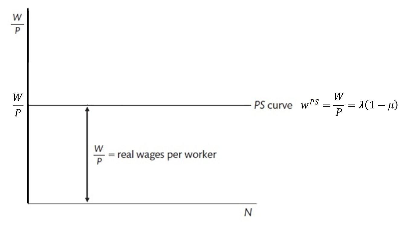
• Rearrange to get W^PS = W/P = 1/(1 + μ)λ ≈ λ(1 - μ)

  • This allows us to put it in W/P - N (Real wage - Employment) space

• Could be conversely understood as a function of markup and price-push factors, W^PS = λf(μ, z_p)

Graphical interpretation of the PS curve

• A horizontal PS curve occurs if marginal productivity of labour is constant (ie, = average product of labour)

• Vertical distance between the PS curve and the horizontal axis are real wages per worker

• If λ is higher on the than the real wage, the vertical distance between the lines is the real profit per worker (μλ)

What causes shifts in the Price-Setting curve?

• Because it is drawn in real wage-employment space, upwards price pushes will shift the PS curve downwards because it’s in the denominator of the y-axis, W/P

• A rise in the tax wedge shifts PS down (tax wedge = real consumption wage minus real product wage, increase in taxes on labour which is shifted onto consumers), a rise in markup and a fall in productivity shift the curve downwards, pushing prices up

Price changes modelled in the PS curve

• P = (1 + μ) W/λ

• Taking logs, logP = log(1 + μ) + logW - logλ

• Differentiating, assume μ is constant, dlogP/dt = dlogW/dt - dlogλ/dt

• = 1/P · dP/dt = 1/W · dW/dt - 1/λ · dλ/dt = ΔP/P = ΔW/W - Δλ/λ

• Such that price growth = wage growth - productivity growth

• When productivity of labour is a constant, a change in wages is equal to the change in prices

Combining the wage-setting and price-setting curves to create the Phillips Curve

• Wage-inflation: (ΔW/W)_t = (ΔP^E/P^E)_{t - 1} + α(y_t - y_e)

• Price-inflation: (ΔP/P)_t = (ΔW/W)_t - (Δλ/λ)_t

• Wage-setters set wages in accordance with last periods price inflation, to which price-setters respond by changing their price to ensure their markup remains fixed

• Assuming there are no changes in productivity, prices rise in line with wage increases/demands

• Substituting wage-inflation into price-inflation, we get:

  • (ΔP/P)_t = (ΔP^E/P^E)_{t - 1} + α(y_t - y_e), where there is no productivity variable because it’s assumed to be 0

    • This can be simplified as π_t = π_{t - 1} + α(y_t - y_e)

Graphical understanding of the Phillips Curve

• In inflation-output space

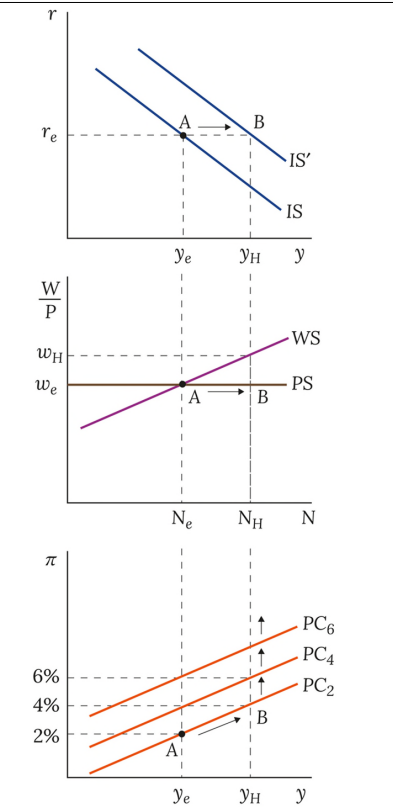
• A positive AD shock shifts the PC upwards increasing employment and worker bargaining power, meaning a wage-setter chooses a higher nominal wage to cover the output gap (higher on the WS-curve)

• Price-setters respond by increasing prices to cover higher nominal wage costs, keeping real wages constant

A positive AD shock without policy response in the current model

• The IS curve shifts rightwards, intersecting the wage setting curve at a higher nominal value and causing an upwards shift in the Phillips Curve

What assumptions can influence inflation expectations?

• The general form might be characterised as π_t = π^E + α(y_t - y_e)

• Adaptive expectations: π_t = π_{t - 1} + α(y_t - y_e)

• Anchored expectations: π_t = π^T + α(y_t - y_e), where π^T is inflation targeted by the CB

The Inverted Phillips Curve

• In terms of output rather than inflation, with an ‘inflation gap’ existent

• y_t = y_e + 1/α · (π_t - π^E)

• The Phillips Curve is the constraint the CB has to operate with when optimising its choice of inflation and output

Graphic interpretation of the WS curve

• Real wage, W/P on the y-axis, Employment on the x-axis

• Labour-force = Natural rate of employed + Unemployed, L = N + U; unemployed is just ‘structural’ or ‘frictional’ which exists regardless of demand

• Labour supply curve is an inverted L-shape (perfectly competitive, typically just vertical)

  • Vertical at ‘full employment’, horizontal is the opportunity cost of working (reservation wage = unemployment benefit + net nonpecuniary disutility of work)

    • It is assumed that everyone’s disutility of work is the same

• Wage-setting curve is effectively a labour supply curve under imperfect conditions (like efficiency wages, bargaining power imperfections)

• Non-intersection of WS and Labour Supply implies a level of employment above structural unemployment due to efficiency wages

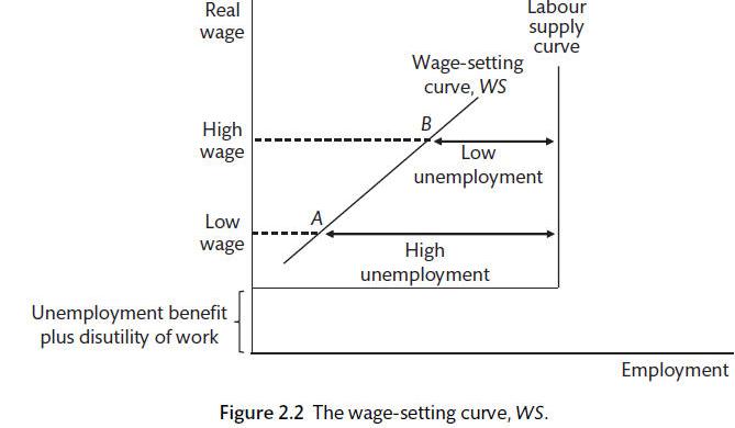
Demand shocks in the Wage-Setting Curve

• A demand shock is effectively an output shock, meaning a rise in income and a positive output gap; the rise in income is correlated with a rise in employment

• There is a reduced cost of job loss meaning a higher wage is required to incentivise workers putting upwards pressure on nominal wages; unions can only demand a higher nominal wage because they don’t control prices

Type of costs incurred in periods of inflation

• Shoe-leather costs: The costs incurred by holding cash during inflationary periods and needing to spend more time managing one’s financial assets

• Menu costs: The costs incurred on businesses when they must frequently review and update their prices (as in literally changing prices on a menu)

Why is low-level inflation targeted?

• To ‘oil the wheels’ of the labour market; it allows firms the flexibility to make real wage reductions without changing the nominal value, thus avoiding frustration generated by apparent wage-change

What does the MR (monetary rule) curve show?

• It shows the chosen output gap (inflation level) of the central bank for any shock; it shows the path along which the CB tries to guide inflation levels back to target

Deriving the MR curve graphically

• Define CB utility in a Loss function, L = (y_t - y_e)² + β(π_t - π^T)², where β is the relative weight attached to inflation; a higher β characterises a more inflation-averse CB

• The Phillips curve acts as a constraint on what employment-inflation level a CB can choose, with many Phillips curves intersecting the Loss function, representing different levels of target inflation; where π_t = π^T, it pass through the bliss point at the centre of the loss function

• The MR curve is derived by identifying and joining the tangency points between the Phillips curves and the loss function

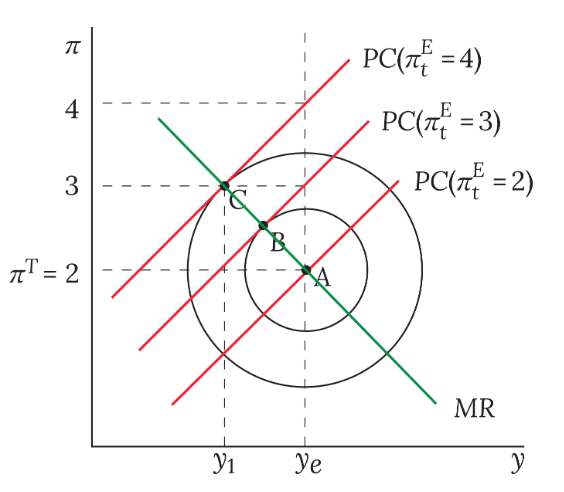
Graphical interpretation of the loss function

• A β>1 means inflation averse, meaning that the loss circles will be squat to account for a smaller range of inflation deviation, whereas unemployment averse will be taller and skinny to allow for less unemployment deviation

Writing the MR curve

• (y_t - y_e) = -αβ(π_t - π^T)

• This is different from a Taylor rule because it expresses a policy response in terms of choosing an output gap rather than choosing an interest rate

Deriving the MR curve mathematically

• Minimise, L = (y_t - y_e)² + β(π_t - π^T)², subject to the Phillips curve constraint, π_t = π_{t - 1} + α(y_t - y_e) with respect to y_t

• Obtain (y_t - y_e) = -αβ(π_t - π^T)

The effect of anchored expectations

• When there is a temporary demand shock, inflation will readjust and no policy response is required; expectations are less anchored as the shock is more sustained

• A permanent demand shock leads to a shift in the IS curve

The deflation trap

• Fisher equation, i = r + π^E

• There is a zero lower nominal bound on interest rates, meaning sometimes the CB can’t set a rate low enough to combat deflation

• Thus, deflation continues and expectations don’t improve, causing a trap; we must resort to fiscal policy or quantitative easing to mitigate the problem

The Fisher equation and finding the policy rate

• r_t^E = i_t - π^E_{t + 1} with adaptive expectations, then the inflation rate of the next period is just expected to be the inflation rate of the current period, π_t

Forecasting the IS curve

• Since the IS curve components target output in the next period, y_t+1 = A_t+1 - ar_t, current interest rates are not linked to current output

• Thus, the CB must set the nominal interest rate to achieve the real interest rate which they forecast will generate their preferred output gap

  • It is central to recognise that there is a lack in the transmission mechanism of monetary policy

How sensitivity parameters affect policy response

• Both α and β affect the MR curve; if either of them is higher (sensitivity to the output gap and inflation respectively) then the MR curve will be flatter

• Reiterating, β>1 leads to a higher compensatory output reduction after an inflation shock

• A higher α (steeper PC) means inflation is more responsive to output, so cutting output decreases inflation by more

• If β>1 then the CB is more inflation averse, leading to a flatter MR curve (in line with the more squat iso-loss curves, which involves a sharper cut in output to response to a shock)

Slopes in the TEM

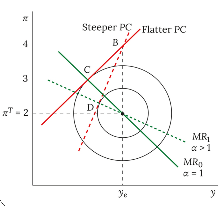
Components influencing policy response

• π_t: shifts the MR curve

• y_e: shifts the MR curve

• β: sensitivity to inflation deviations, affects the iso-loss curve shapes and slope of MR

• α: sensitivity to output gap deviation, affects PC and MR slopes

• a: interest sensitivity of investment, alters IS slope

Stabilisation Policy in the TEM

• After an inflation shock, the PC shifts up to a new place on the PC

• CB forecasts the PC for the next period and picks the optimal point on it (where it intersects the MR curve) which decides the interest rate it must adopt to move the economy back to the equilibrium level

Impulse response functions

• On the y-axis is value of the variable and on the x-axis is time, to measure how the variable changes with respect to time

• Use them whenever using the TEM to show understanding of how the variables change over time

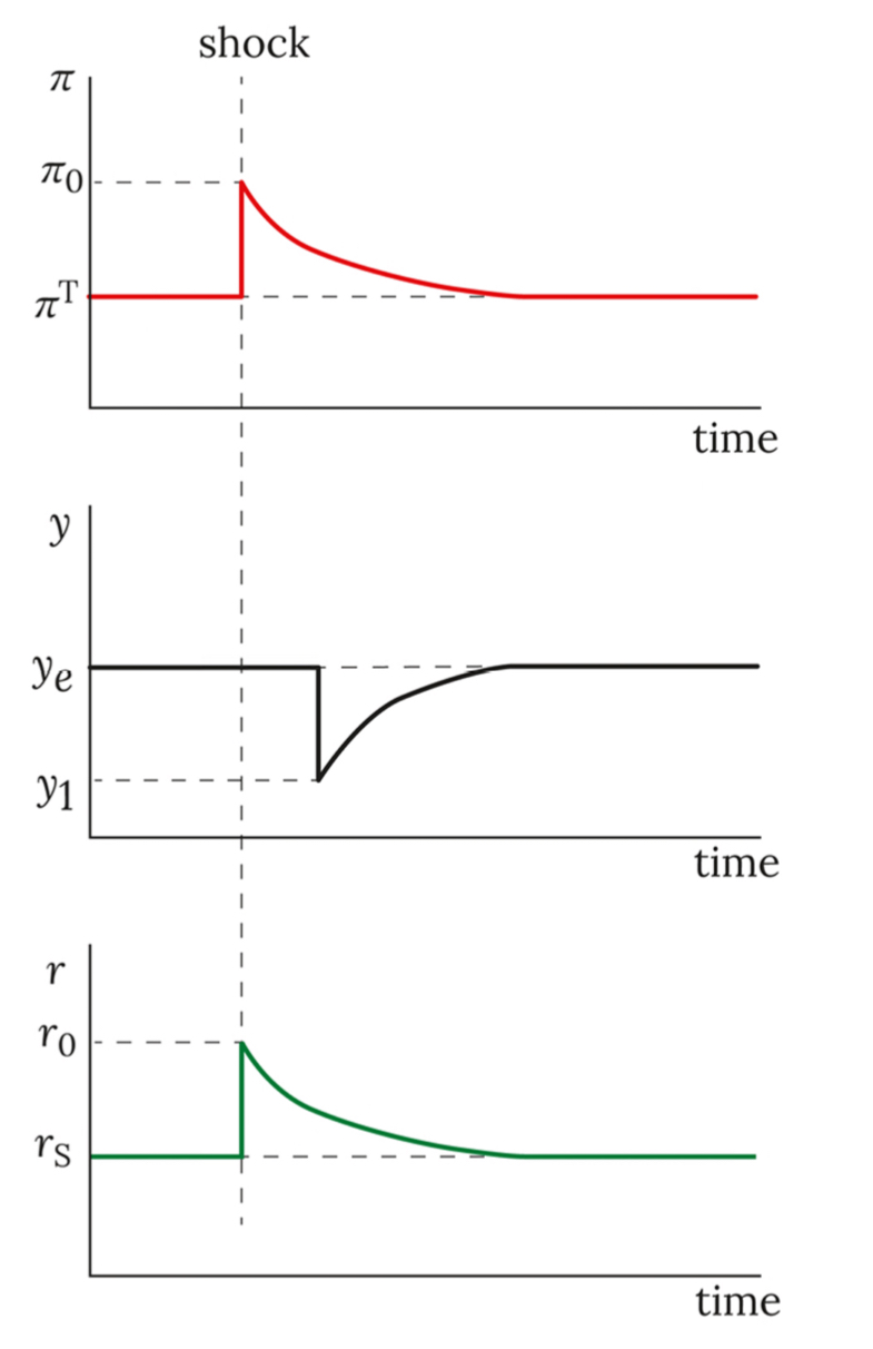
Effect of a permanent demand shock

• In the absence of a policy response, inflation expectations remain high leading to increasing inflation

• The IS curve shifts and thus the PC also moves up continually unless the CB changes AD by altering the interest rate

• Even after all the interest changes, we return to equilibrium output and inflation, but we never return to the initial real interest rate which is increased permanently

What are the different types of monetary policy rules?

• Taylor Rule, Balanced Approach Rule, Balanced Approach (Shortfalls) Rule, Adjusted Taylor (1993) Rule, and the First Difference Rule

• Each one shows a different monetary policy response, with slightly different weightings on inflation and unemployment deviations

• The adjusted Taylor (1993) rule is the only one which recognises that the FFR can’t be set materially below the effective lower bound

  • It proposes changing the interest rate only after the economy has begun to recover

Limitations of different policy rules

• Often tested in conditions which have less variables and are unlike the actual conditions the FOMC considers, meaning their results often abstract away from real conditions

• They also often do not take into account the effective lower bound on interest rates

• Simply policy rules also don’t take other monetary policy tools into account, like balance sheet policies

Policy rule prescriptions in the pandemic

• All of the simple monetary policy rules allowed for a very accommodative stance of monetary policy in response to pandemic inflation pressures

• For most of 2022, the rules prescribed a rate between 4 and 8 %, which was much higher than the levels actually observed in the pandemic, perhaps due to elevated inflation readings

  • For most of 2022, the actual target range for the FFR was below the prescribed policy rates, but this gap has lessened as the FOMC has tightened the stance of monetary policy

What is Taylor’s rule?

• A policy rule created by John Taylor in 1993 which describes the FED reserves interest rate choices

• It is given as i_t = π_t + r_s + 0.5(π_t - π^T₎ + 0.5(y_t - y_e),

  • or conversely as r_t - r_s = 0.5(π_t - π^T₎ + 0.5(y_t - y_e)

• Where i_t is the nominal interest rate, r_t is the real policy rate, r_s is the stabilising real interest rate; Taylor used r_s = 2% in the long run rather than a varying one

What is a stabilising rate?

• Denoted by the subscript s, this leads to an economy at equilibrium (y_e, π^T)

• They are related by the Fisher equation, i_s = r_s + π^T

What is the CB policy rate called?

• The Federal Funds Rate

How is the Taylor Rule implicit in the TEM

• PC// π_t = π_t-1 + α(y_t - y_e), MR// (π_t - π^T) = -1/αβ (y_t - y_e), IS// (y_t - y_e) = -a(r_t-1 - r_s)

• Substitute π_t from PC into MR, substitute (y_t - y_e) into MR

• Rearrange to get r_t - r_s = 1/a(α + 1/αβ)(π_t - π^T), the TEM Taylor Rule

Comparing the Taylor Rule with the TEM Taylor Rule Mathematically

• r_t - r_s = 1/a(α + 1/αβ)(π_t - π^T) is TEM, normal Taylor Rule is r_t - r_s = 0.5(π_t - π^T₎ + 0.5(y_t - y_e)

• γ(π_t - π^T), where γ = 1/a(α + 1/αβ)

  • Where α = β = 1, then the TEM Taylor Rule becomes r_t - r_s = 0.5(π_t - π^T)

• This is now an optimal response rule rather than an ad hoc proposition

How do the TEM Taylor Rule and the normal Taylor rule differ?

• In the TEM version, there is no explicit output gap term such that optimal responses only concern inflation deviations

• This is because the TEM implies a linear relationship between inflation and output

• Taylor’s Rule has no formal theoretical derivation, it has simply worked empirically, and it is more general, suggesting how a CB should respond to an output gap even if they’ve already responded to inflation

What is meant by coefficient variation in relation to the Taylor rule?

• Most CB have dual mandates of unemployment and stable inflation, but some weight them differently, like the Bank of England which cares more about price stability

• r_t - r_s = ψ(π_t - π^T₎ + ψ(y_t - y_e) is a more general representation of this rule

  • Castro (2011) measured the extent to which different CB’s targeted different components, where the research suggested coefficients of 1.53 and 1.40 for price stability and unemployment in the FED respectively, the BoE was 1.87 and 0.99 respectively and the ECB 2.77 and 1.99

How can the Taylor Rule lead to unachievable recommendations?

• During crises, the Taylor rule has often proposed negative policy rates, which many countries cite, as a rule, cannot go below 0 (they could go below 0 practically, but it would be administratively strenuous)

• Central Banks can occasionally set slightly negative policy rates because, due to the costs of holding cash, financial institutions will buy short term securities and bonds at prices which imply negative yields

  • Hence the lower bound is an effective lower bound

What is the Taylor Principle?

• Any monetary response to an inflation shock should reduce the adverse effects of the inflation

• Parameters of the Taylor Rule must obey to guarantee that a monetary response is sufficient to counter the shock

• Using the Fisher relation, the Taylor principle can be shown to imply that the rise in the (nominal) policy rate must exceed the rise in inflation that results from the shock

• This principle holds regardless of the type of Taylor rule implemented

What is quantitative easing?

• An unconventional monetary policy rule involving the outright purchase of government bonds or financial assets by the Central Bank

• These bonds could be already existing or created new for this

• UK quantitative easing involved the buying of existing bonds

• Bond purchases are funded by the creation of reserves at the Central Bank

  • Reserves are accounts held at the CB which make up Base Money — these reserve accounts are extremely liquid

Quantitative easing methods

• BoE created CB money and used it to buy gilts (UK government debt) and eligible corporate bonds from private investors in secondary markets

• Bonds were sold through reverse auctions (pre-announced prices and assets)

• Transactions were facilitated by trusted intermediary counterparties like banks who hold reserves at the CB

• Assets bought during QE are held at the Asset Purchase Facility (APF)

What are gilts?

• UK government bonds which are essentially debt where interest is paid on sums borrowed from bond-owners

• Market price is quoted in terms of price per £100 face value (as a percentage)

  • Bonds aren’t traded at face value because price varies with the interest rates available in the money markets

• The amount of interest paid is called the coupon rate and this is often paid semi-annually to make up the total account over the year

• At maturity a person holding the bond receives the principal value back

The Asset Purchase Facility

• Holds both the security and the debt from buying the security

• Increases in the interest rate means that bonds lost value such that the assets held are worth less than the debt accrued

How are interest rates and bond prices related?

• They are inversely related meaning as interest rates increase the price decreases

Why might the CB transact gilts?

• Gilt purchases might be used to adjust the quantity of reserves to target an ideal policy rate in Open Market Operations (OMO’s)

• Gilt purchases might also be used to influence long term interest rates

Operational Standing Facilities

• BoE operational standing facilities (OSF) allow trusted counterparties to interact with the CB directly (depositing or borrowing)

  • These are often short term

• The spread between OSF lending rate and OSF deposit rate has been reduced from 25 basis points to 15 in 2025 to ensure better market functioning

What does QE lead to?

• An increase in reserves which are part of monetary base (reserves aren’t broad money because it is not used for spending)

• Reserve creation only occurs when the CB buys an asset from the private sector, it is not a transfer of wealth, rather it is an asset swap

  • BoE removes gilts and simply puts reserves in the private market (one interest-bearing claim out for the other)

Aims of QE

• The primary aim of QE is to reduce yields, NOT to create more money

• QE affects the economy only to the extent that it affects interest rates, which is the only form of conventional monetary policy which works

• These are the arguments given by CB

• The ultimate aim was to make it cheaper for households and businesses to borrow money

  • If the increase in money had been enacted through other means such that it was an injection of spending money into the economy, then there might be pent-up or exaggerated inflation

Timeline of QE in the UK

• Monetary policy of the CB is to maintain price stability (2%)

• It can determine this by setting the Bank Rate and by using QE

• In 2009, CB bought £200b gilts

The effects of QE

• QE1 had a large effect, reducing market interest rates

• QE2/3 were smaller and more predicted such that there was very little effect on interest rates

  • Much of the same is true for QE4

• QE5 had a large effect due to the vast amount of asset purchases, inducing sufficient surprise that interest rates were reduced

Intuitive explanation for why QE works?

• Lowers effective interest rate/yields such that investors rebalance their assets by purchasing riskier assets, which itself contributes to the interest rate on loans being reduced

  • More expensive bond price acts as a signal to other interest rates in the market

• It makes it cheaper to borrow money and therefore encourages spending

  • Simply, they buy bonds to push interest rates down to encourage borrowing/spending

    • Bond purchase reduces supply, meaning that bond prices go up which is inversely correlated with yields and interest rates

When is QE implemented?

• There is no further scope for conventional monetary policy (ie, interest rates are already at the zero lower bound)

Effects of QE on the yield curve

• It cannot change the short end of the yield curve — this is already at the lowest amount any institution would trade them at

• It aims to raise the price and thus reduce the longer-term yield of the bonds, signalling a pivot of the yield curve to make it flatter

• In this case, i_s refers to short-term interest rates

• In the case where the zero lower bound is reached, i_L is still too high — bank lending is a long term process, so this long-term nominal rate must be reduced somehow to ensure movement away from the ZLB

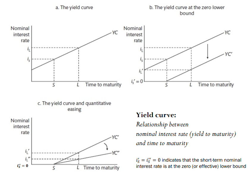
Why does QE neutrality suggest that QE shouldn’t work?

• This view asserts - under the core assumptions of many finance textbooks - that QE bond purchases would not affect yields at all so the yield curve would not pivot

  • These assumptions include no frictions (preferred habits), no credit or liquidity risk, implying assets only have pecuniary values and can be bought in arbitrary amounts

• This means investors are happy to hold assets of any maturity such that they are indifferent between holding reserves and short/long-term bonds (the only thing which gives an asset its value is its rate of return)

• Therefore, APF bond purchases do not affect investors portfolios and QE should have no effect on the yield curve unless QE acts as a signal about future interest rates

QE transmission diagram

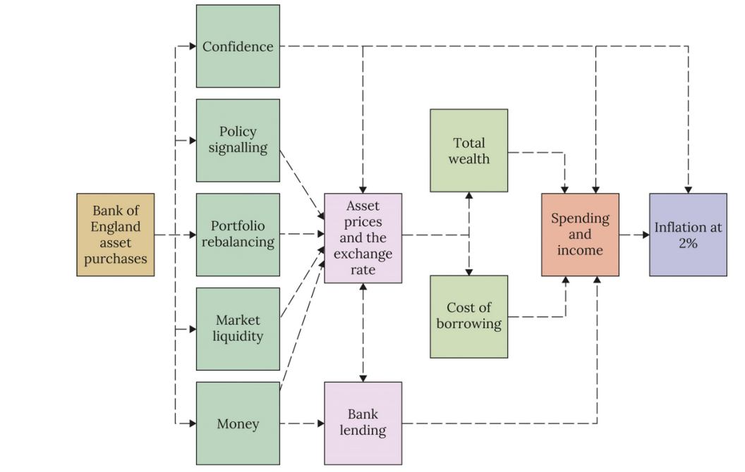
How do different QE transmission channels work?

Portfolio rebalancing:

• Money from bonds sold to CB can be used to purchase other financial assets, decreasing yields

  • The bank of England primarily cites this channel as its justification for using QE

Liquidity, market functioning, confidence, uncertainty:

• Directly affects asset prices, boosting liquidity and encouraging trading

Signalling:

• QE demonstrates that a commitment to target inflation helping to anchor inflation expectations and avoid a deflation gap

How does the portfolio rebalancing view violate QE neutrality?

• It ignores the notion that investors don’t have preferred habitats (a preference for a particular maturity bond) — a habitat is a section of market participants

• Will only have an impact if there are some inefficiencies in the market and investors won’t view reserves as a perfect substitute for bonds

Do preferred habitats exist?

• Yes. In the UK government bond market investors tend to prefer bonds with particular maturities

• These preferred habitat investors are often less price-sensitive than other investors

The ‘local supply’ channel of portfolio rebalancing

• QE can reduce the yield and raise prices of other assets because preferred habitat investors are content to hold bonds even when their yield slightly decreases

• They will also sell bonds through quantitative easing and use reserves to buy other assets, in turn pushing their prices up

The ‘duration effect’ channel of portfolio rebalancing

• QE reduces the yield of long-term assets skewing favour towards short-term assets (with lower duration risk), meaning markets shift towards short-term assets with lower risk

  • Hence, overall expected returns should rise

What is duration of a bond?

• This is measure of sensitivity of a debt instrument to interest rate changes

• The higher a duration, the more the bonds price will drop as interest rates rise

• Duration depends positively on the maturity and negatively on the coupon rate

  • Basically, a bond with a longer maturity has a greater interest rate risk

Limits of the portfolio rebalancing channel

• It requires that there is limited arbitrage — other investors can’t act to undo other people’s previous investment actions, like preferred habitat investors

• They might not do this in the absence of market imperfections because of financial constraints or risk aversion

The signalling channel of QE

• Asset purchase acts as a signal from the CB to say that it will keep its policy rate low for a long time, in turn lowering future interest rate expectations

• QE can act as a commitment about interest rates or alternatively can act as an indication about the state of the economy

How can QE act as a commitment about interest rates?

• QE makes it costly for the CB to raise interest rates once inflation rises above target, meaning that it has less incentive to deviate than if it just made a simple promise

• This helps to solve the time-inconsistency problem

• However, in the UK, HMT has indemnified the CB against balance sheet losses, so these losses would have no real effect

Liquidity, market functioning, and uncertainty channels

• Promise to buy bonds ensures market participants they could sell theirs if they wish, reducing the liquidity premium (yield = risk free rate + liquidity premium)

  • This is reduced because BoE offers to buy long term bonds for short term liquidity (reserves)

• This channel seems to depend on market friction or quantity constraint - when liquidity is in demand

• Interaction between portfolio rebalancing and the liquidity channel could occur

What is the quantity theory of money?

• Concerns different factors which pin down the real and nominal aspects of the economy (output, employment, vs price level, inflation rate)

• Py = MV, where P is price level, y is output, M is the money supply, and V is the velocity of money circulation; each variable is often expressed in terms of growth rates

  • Under the assumption wages and prices are always perfectly flexible, M pins down P which pins down real inflation

What is the monetary base multiplier?

• k = (1 + cd)/(cd + rd), where cd is the cash-deposit ratio of agents and rd is the reserve-deposit ratio of the CB

• However, there is debate as to whether this equation accurately represents any real relationship

Policy response under the Taylor Principle

• Where the general form is r_t - r_s, r_t = i_t - π_t and r_s = i_s - π^T, the Taylor rule can be written as i_t - π_t - (i_s - π^T) = ψ₁(π_t - π^T) + ψ₂(y_t - y_e), so the general Taylor rule in terms of nominal policy rate is i_t - i_s = (1 + ψ₁)(π_t - π^T) + ψ₂(y_t - y_e)

• The Fisher relation shows that an increase in π_t requires a nominal policy response to reduce investment — in the Taylor rule, expressed in terms of real rate, this implies that ψ₁ > 0 to ensure an adequate response, thus, (1 + ψ₁) > 1, implying the change in policy rate must be greater than the increase in inflation

• It is important that the real and nominal interest rates respond positively to the output gap

What is the yield curve?

• It plots the yields on bonds of differing maturities against the time until maturity (nominal interest rate on the y-axis)

• An upwards-sloping curve means yields on longer maturities are greater than those on short-term maturities, consistent with expectations that the nominal rate will rise in the future

  • This might also reflect a term premium that comes with holding an asset for longer - it is more vulnerable to shocks and unexpected events

    • It is often assumed that this risk premium is non-existent to understand how bonds can convey monetary policy expectations

How are returns on bonds calculated?

• If markets are efficient, the returns on a 5 year bond is the geometric average of the expected and actual returns of a series of one-year bonds held for five consecutive years

• Total return = (1 + i_1t)(1 + i^E_1t+1)(1 + i^E_1t+2)(1 + i^E_1t+3)(1 + i^E_1t+4) = (1 + i_5t)⁵

  • Numerical subscripts indicate bond maturity, ^E represents a nominal rate expectation, and _{t, t+1} etc represent the time of purchase of the bond

• A 1-year maturity just reflects the short term interest rate in the period (ie, t → t+1)

What is the conventional monetary policy transmission mechanism?

• How changes in the bank rate alter the economy-wide inflation level

• Changes in the bank rate first filter through the financial markets as interest rates are affected and rates of borrowing influenced by the rate one can borrow at from the CB

• Money market changes affect asset prices and the exchange rate, which filters into the labour market, influencing wage-setting and price-setting curves and eventually influencing prices

• This process is subject to influence from outside shocks like fiscal policy, changes in global economy, and changes in commodity prices

What are the 4 main channels of conventionary monetary policy transmission?

• Market rates → a reduction in i_t makes borrowing desirable, increasing AD

• Asset prices → lower i_t increases asset prices, increasing household wealth and spending (increase in autonomous consumption)

• Expectations → decrease in i_t shows CB commitment to monetary policy

• Exchange rate → decrease in i_t increases nominal exchange rate e, increasing the real exchange rate Q, therefore increasing exports over imports (X - M), increasing AD

Conventional vs unconventional monetary policy

• Conventional alters the short-term interest rate, whereas unconventional policy like quantitative easing target the long-term interest rate

• Conventional monetary policy alters short-term nominal rates and buys short term bonds → investors cares more about long-term rates

In what way is quantitative tightening (QT) just unwinding QE?

• MPC decides whether QT is passive or active — passive involves not reinvesting the funds from maturing bonds whereas active involves selling these securities on secondary markets

• If active is pursued, the MPC decides an annual amount of bonds sold

• Even if not sold, passive QT would lead to a reduction in the stock of Gilts as the bonds mature

QT decisions made in the UK

• BoE stopped buying bonds at the end of 2021 and stopped reinvesting the proceeds in February 2022, announcing bond sales would occur soon after

• Began actively selling bonds in the market in November 2022

• By September 2024, £100 billion reduction in gilt stock, with the plan to sell £70 billion worth between September-October 2026

  • Decision to sell Gilt stock was put down to a vote in the MPC, with a 7-2 in favour of the 25/26 policy

What is GEMMD?

• Gild edged money market dealers are old financial institutions which act almost as intermediary dealers of bonds

How does UK QT compare with the rest of the world?

• Other major CB generally only engage in passive QT (like the FED, ECB)

• The Reserve Bank of New Zealand were the first country to engage in active QT

Potential downsides of active QT

• QT in the UK via sales to secondary markets has the potential to disrupt gilt markets

  • It’s easier in New Zealand gilt markets because they only have a small stock of gilts in the first place, making it more absorbable

• Also, the gilt market might struggle to absorb QT gilt sales alongside new issuance from the Debt Management Office (DMO)

• So, UK fiscal policy + QT requires the private sector to absorb historically high volumes of public debt over coming years, equivalent to an increase in private sector holdings of public debt of 6.4%

What are the upsides of QT?

• It might provide financial stability by reducing cases where the Bank owns high proportions of particular maturity gilts, evening out the supply of bonds in the market

• Active QT doesn’t change the payment of coupons on gilts (still paid, but to the private sector), but it does reduce interest payments on reserves because they are now held at the government again

  • In 2023, interest payments on reserves amounted to around £30 billion (slightly inflated) and HMT (tax) pays this if the APF is making net loss

    • It is suggested that interest payments can contribute £6.7 billion to annual deficit

Why did the MPC choose active QT?

• Reduce large gilt holdings to allow for future QE

• Without selling long-term gilts, the UK would be very protracted, still holding £400 billion in 2034 and lumpy, since the volume of maturities would fluctuate from month to month and year to year

  • Handelsbanken plc calculated that “Without active QT, there would have been no QT taking place from October 2022 all the way until July 2023” (Treasury Committee of UK parliament)

QT in the context of monetary policy

• QT is not an active instrument of monetary policy is meant to be the nominal interest rate - this doesn’t aim to respond to macroeconomic conditions

  • Despite not being an active instrument, it may have contractionary effects

• There is still substantial uncertainty about the effects of quantitative tightening

Asymmetries between QE and QT

• It is not QE in reverse, it is not designed to tighten monetary conditions

• It is conducted when financial markets are calm, whereas QE is a means of alleviating market disruption and stimulating economic change

• There is also a distinct lack of a signalling channel for QT, whereas QE signals limits of conventional monetary policy and demonstrate a commitment to a rate

• Additionally, liquidity and market operation channels don’t operate for QT → the only one which could be feasibly maintained is the portfolio rebalancing channel

Why can’t base money be spent?

• It is only accessible by certain financial institutions and is used to settle accounts between Central Banks and financial institutions

Where do reserves go in QT

• Reserves simply vanish once gilts are returned to the private sector

• The CB wants to reduce reserves despite being able to create as many as they want — the size of it and the unusual nature of the balance sheet is alarming to bankers

Effects of QT on the slope of the yield curve

• Active sales back into the secondary market is likely to reduce bond prices and raise yields

• It provides more duration to secondary markets, meaning that as interest rates rise, bond prices are likely to drop more for long-term bonds than for short-term bonds

• The short end of the yield curve is pinned down by the policy rate, so any QT impact will affect longer maturities — the yield curve might pivot anticlockwise