Univariate Statistics Quiz 1

Variable

able to vary, anything that can take on different values for different observations

Constant

something that does not vary, static across observations, no change

Levels

the values that a variable can take on (ex. different ages being the level of the variable of age)

Nominal

(name) a variables level are different only in name (ex. eye colors, birth states)

Ordinal

(inherent order) levels also have a natural order, no sense of how much difference or scale there is between them (ex. military rank, soft drink size)

Categorical values

nominal and ordinal

Interval

(consistent interval) unit interval always means the same thing, a unit has a meaning, there’s a scale, unlike ratio (ex. temperature, calendar years, time of day)

Ratio

the value zero means “none”, allows calculations of ratios that make sense (ex. age, amount of money in pocket)

Continuous values

interval and ratio

Populations

often too big to measure, instead select a subset of the population to pull out and measure, the set of all possible scores

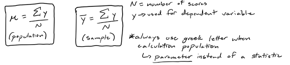
Parameter

summary value that describes a population

Sample

the subset of the population that is actually measured, goal of the sample is to understand the population not just the sample, a summary value described using statistics

Statistics

summary values that describe samples, used to estimate parametersIn

Inferences

drawing conclusions about a population based on what is observed in a sample, importance of the idea of random selection to work with a representative sample of the population

Descriptive statistics

anything that meats the definition of a statistic, wanting to describe the thing that we observed, values meant to describe the data measured, have a UNIT used to describe them (ex. the mean of a sample (range of scores), average)

Descriptive parameters

can describe the population based on descriptive statistics

Test statistics

doing a test to compare statistics, gives a value to find a difference, used to make decisions, don’t help to describe what was in the sample, NO UNIT, only exist in samples not in parameters (ex. z, t, f)

Independent variable

causes

Dependent variable

effect, dependent on the IV

Selecting an analysis

Mean

can be sensitive to extreme scores

Median

The middle score in a set of ordered scores (the score with the same number of values above and below)

Mode

• "where are scores most likely to be"

• Most frequently occurring score

• Most frequently occurring interval (histogram)

  • Histogram - break up number line into intervals (used in lab 1)

• Score with highest probability density (top of the curve)

Range

• max(y) - min(y)

• Difference between the highest and lowest value

  • Limited while only describing two points in the data set

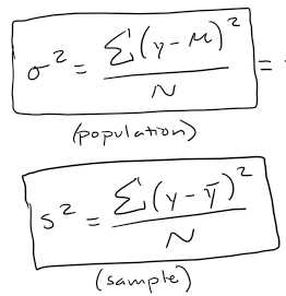
Variance

Average of the squared differences between score and population mean

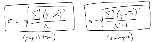
Standard deviation

Square-root of variance (back to the variable's original metric)

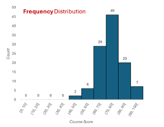
Frequency distribution

• Heights of bars represent counts for the number of scores within each interval

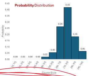
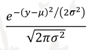
Probability distribution

• Showing the scores in each interval as a proportion of the larger total number of scores

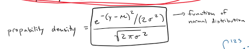
Probability density

used to describe the independent variable, integral to find area under curve to find probability

whole curve is the data, integral to find the probability of pulling a score from that certain range

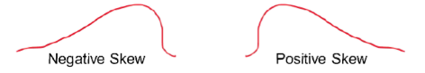
Skew

asymmetry (the normal distribution is symmetrical)

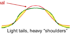
Leptokurtosis

more peaked than a normal curve

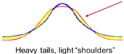
Platykurtosis

 flatter than a normal curve

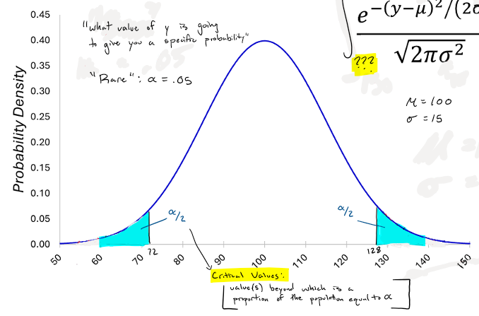
Definition of rare

alpha = .05

Distribution based probabilities

• find probability within a specific range using an integral

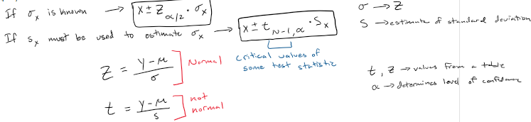
Critical values

value(s) beyond which is a proportion of a population equal to alpha

“what value of y is going to give you a specific probability”

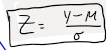
Standardizing equation

Z, simplified metric easier to understand

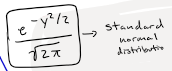
Standard normal distribution

Point estimates

specific point on the number line, precise, almost always wrong (at least a little)

no confidence that it’s the right answer

(ex. 5.7)

Confidence interval

less precise, much more likely correct

(ex. [5.4,6.0]

“Confidence”

stated as a percentage

90% confidence means that if a confidence interval is calculated for many, many samples, 90% of the samples’ confidence intervals will include the parameter being estimated

relationship between percent and confidence (C) and alpha

Confidence interval equation with sigma SD known and unknown

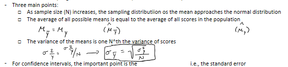
Central limit theorem

describes the sampling distribution of the mean, distribution of sample means

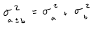
variance sum theorem

for any two unrelated (independent) variables a and b, the following relationship holds:

the variance of the sum or difference is equal to the variance of the sum

Significance testing

 decision making tool to help figure out when we can make an inference

Goal of significance testing

• Decision-making

• Inference

• i.e. deciding whether the observed results are strong enough to support a conclusion that the population from which the sample was drawn is different from the null population

• If results support such inference, they are said to be "significant

Statistical significance vs. practical significance

• Practical significance: a result is big, strong, or important

  • "the temperature dropped significantly over the weekend"

• Statistical significance: a result supports the inference that an effect or characteristic exists in a population

• Effects that are of great practical significance can be statistically non-significant

• Effects that are of very little practical significance can be statistically significant

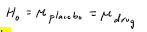
Null hypothesis

the absence of what we are looking for

Data

something we have seen/measures

Target

an effect or characteristic we are looking for

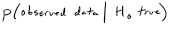
Probability

describes sample relative to null hypothesis

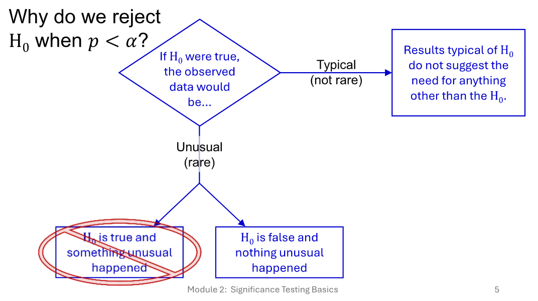
“low” p means” the observed data would be “rare” if the null hypothesis was true

Plum tree example:

• We are tying to find a plum tree (target). Observe a tree with purple fruit

• Null hypothesis (H): this type of tree is not a plum tree with purple fruit

• Purple fruit would be rare among non-plum trees (if H were true, the observed date would be rare)

• Conclusion: we reject the not-a-plum-tree idea (reject H) and conclude that we have found a plum tree (assume that the null hypothesis is right until proven wrong)

  • Focus on knowing what we know that the thing you're looking for does not exist or isn't true

Significance testing procedure

1. Define "rare" as an arbitrarily low probability (usually alpha = .05)

2. Specify a target - what are we looking for?

3. State the null hypothesis

4. collect data

5. Find the value of a test statistic (z, t, etc.)

6. Use the test statistic value to find a p-value or critical value

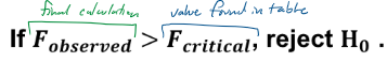
7. Decide: if p<a (or if, e.g. z(observed) > z(critical)), reject H

8. If H is rejected, describe result as "significant" and use descriptive statistics to describe the (estimated) population. E.g., "Symptom Severity is significantly lower among those who received the drug (ybar = 19) than among those who received the placebo (ybar = 73)

   1. If rejecting then null hypothesis, that means that you found what you were looking for

Why do we reject the null hypothesis when probability < alpha?

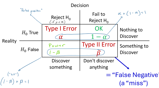
Outcomes: type I error, type II error, power, “ok”

Type I error:

• reject null hypothesis, reality that null hypothesis is true

• “false positive”

Type II error:

• don’t discover anything, something to discover

• “false negative”, a miss

power:

• reject null hypothesis, reality that null hypothesis is false

• “hit”

“ok”: fail to reject null hypothesis, nothing to discover

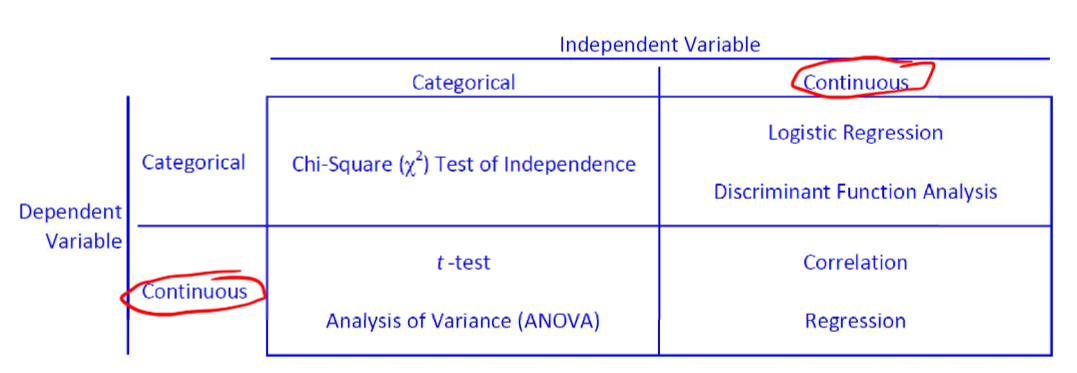
Selecting an analysis

Population variance equation

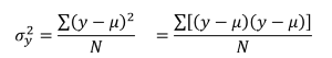
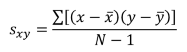
Population covariance equation

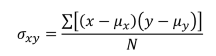
Sample covariance equation

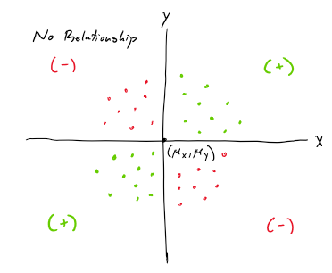
No Relationship scatterplot

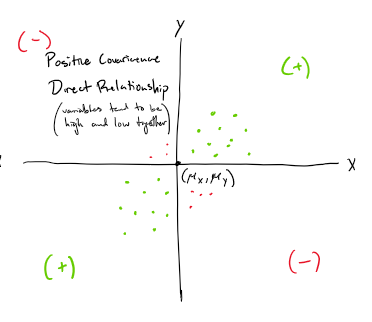
Positive covariance scatterplot

direct relationship

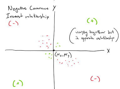
Negative covariance scatterplot

inverse relationship

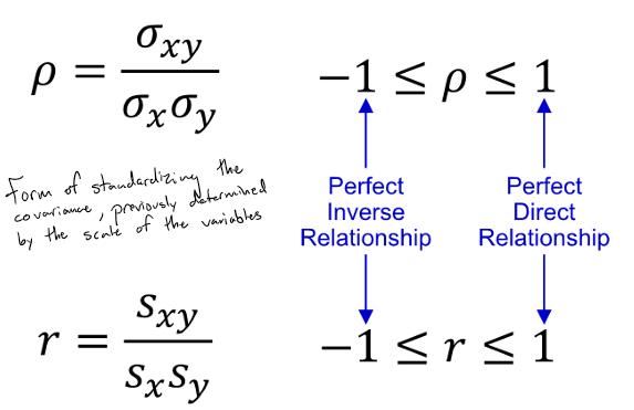
Correlation coefficient

form of standardizing the covariance, previously determined by the scale of the variables

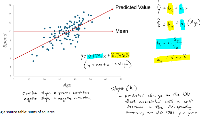
"Predicting" scores" mean vs. regression line

• "I now want to be able to guess how much someone Is going to spend

• Mean is always the best guess in the long run in general

Regression line

procedure of giving us a way to come up with a best guess, the predicted value

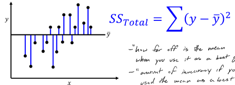
Sum of squares: total

• “how far off is the mean when you use it as a best guess”

• “amount of inaccuracy if you used the mean as a best guess”

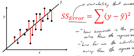
Sum of squares: error

• variability that cannot be explained by the regression model

• “how far are the individual values from the regression line”

• “is it doing better then the mean at a best guess”

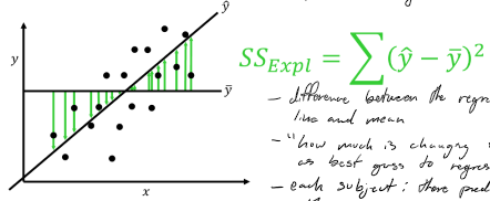
Sum of squares: explained

• difference between the regression line and the mean

• “how much is changing from mean as best guess to regression line as best guess”

• each subject: the predicted value minus the mean

Source table

• MS = mean square (average of the square deviations), another way of saying variance

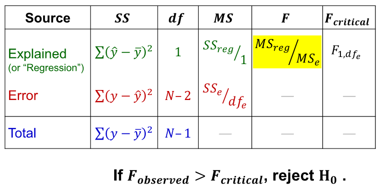
How to use F

F is used to test the null hypothesis, “the IV cannot predict the DV”

Regression assumptions

• Linearity

  • for every line of the IV, all population DV means fall on the same line

• Normality of errors

  • assume that their will be a normal variance of errors

• homogeneity of error variance

  • population variance in the DV is the same for all levels of the IV

• independence of errors

  • no two or more errors are similar to one another because they come from a common source

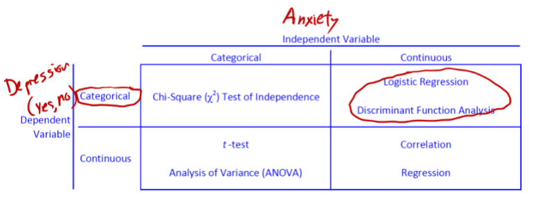
Selecting analysis: IV categorical, DV categorical

chi-square, test of independence

Selecting analysis: IV continuous, DV categorical

logistic regression and discriminant function analysis

Selecting analysis: IV categorical, DV continuous

t-test and/or analysis of variance

Selecting analysis: IV continuous, DV continuous

correlation or simple regression