NRS 305 Final

population regulation

population size and growth are limited by density dependent and density independent factors

density dependent

increasing population size causes per capita growth rate to decrease. example: limited food leads to competition in population

density independent

affects per capita growth rate regardless of population density. example: natural disasters

whooping cranes

low chick survival is a major limiting factor that keeps small population size from growing. Management strategy: increase chick survival

bighorn sheep

predation matters but varies too much in survival and reproductive rates across locations. Management strategy: must be site specific, some populations unaffected while others are struggling

vancouver marmots

very small population sizes to the point little predation is impactful. Management strategy: reduce all mortality sources, even if they seem minor

white sharks

increasing shark populations are linked to increasing seal populations. Management strategy: population regulation involved intricate food webs, must consider entire ecosystems and not just one species

new england cottontails

high predation rates are a major limiting factor during reintroductions. Management strategy: focus on predator control or habitat managements during reintroduction of population

primary focus on top down

humans are predators and see other predators as competition, predators often pose conservation and management issues (white tail deer overpopulation because no predators), anti-predator adaptations (camouflage, porcupine spikes), predators mainly blamed for declining prey populations

White tail deer in Wisconsin

severe winters, multiple sources of mortality (bears, cars, humans), bottom up controls, wolf and deer populations are coincidental, deer populations increases during more mild winters even when wolves present

dP/dt=caRP-dP

lotka volterra predator model

c

LV, capture efficiency of predation

a

LV, efficiency of converting food into predator growth

R

LV, prey population size

P

LV, predator population size

d

LV, predator death rate

LV predator assumptions

predators only eat one species at a time, predator efficiency does not change with prey abundance

dR/dt=rR-cRP

lotka volterra prey model

r

LV, prey growth rate

LV prey assumptions

prey limited only by predators, predator efficiency does not change with prey abundance

snowshoe hare, canadian lynz

rare cyclic relationship between predator prey populations predicted simple models, predicts boom-bust cycles

Lemming cycles

pattern does not fit simple LV cyclic model, population peaks don’t occur in regular intervals, smooth increases and sudden crashes, populations influenced by multiple factors not just predation

support top down control

if lemmings are mainly controlled by predation, then population shouldn’t crash when predators are excluded from the experiment

support bottom up

if lemmings are mainly controlled by bottom up, lemming survival and reproduction rates are higher when more food is added

predator efficiency

the proportion of the prey population that a predator can successfully capture and consumer per unit time, small amount of prey means high efficiency, large amount of prey means less efficiency

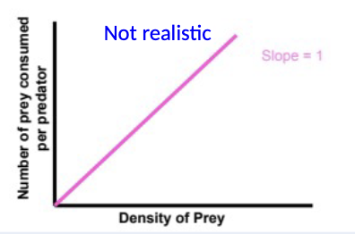
type I functional response

rate of consumption per predator is proportional to prey density (constant slope, no satiation)

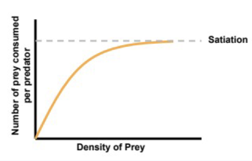
type II functional response

rate of increase in prey consumption per predator starts high, diminished and ultimately plateaus with increasing prey density

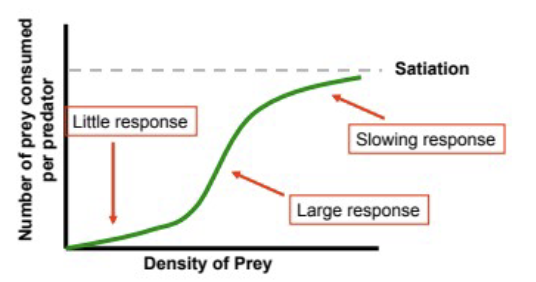
type III functional response

predator response to prey is depressed at low prey densities, then accelerates, then plateaus once reaching satiation

Hen harriers and red grouse

when red grouse populations are low → hen harriers dont focus on them, red grouse becomes more abundant → prey switching, efficiency increases

hen harriers concentrate on red grouse → leads to satiation and efficiency levels off

search image

when a predator begins to recognize and focus on a specific type of prey, increase predator efficiency in functional relationship between predator and prey populations

prey switching

predator switches from consuming one prey to another depending on which is most abundant, functional models assume no prey switching, but as prey population declines predator may switch to another prey species weakening their interactions

immigration and emigration

not included in functional response, assumes populations are closed, may help prey populations avoid crashing, can lead to prey switching

nelson and mech (2006)

wolves heavily preyed on deer in that area → depleted deer populations → wolves switched to new prey, moose → shows prey switching allows predators to persist

territorial behavior

puts a cap on how many predators can occupy an area, predator density cannot freely increase as prey becomes abundant

1910, swam over

when and how did moose colonize isle royale

1948, crossed ice bridge

when and how did wolves colonize isle royale

factors influence moose populations

overbrowsing of balsam fir, malnourishment, ticks

factors influence wolf populations

inbreeding due to low population size

lynx-hare cycle

classic, predator driven, predictable cycles, wolf-moose cycle has lagged responses and irregular cycles in comparison

rmax

isle royale, maximum per capita growth rate of resource recruitment (balsam fir), how fast plant can grow when not limited, represents growing season and climate conditions

k

isle royale, carrying capacity in absence of consumers, max amount of plants environment can support, represents habitat productivity

a

isle royale, area searched per unit time by consumer, how quickly moose can find and consume plants, higher means stronger pressure and less plant biomass

h

isle royale, handling time for each item, limits how much moose can eat, satiation

c

isle royale, coefficient for converting resource consumption into offspring, higher means more offspring per unit food

d

isle royale, consumer per capita mortality rate

a

tri-trophic model, maximum rate moose can eat plants, higher means stronger grazing and reduced plant biomass, represents foraging ability and feeding time

b

tri-trophic model, plant biomass at which consumption is half of maximum, low means moose feeding rates are high even when plants are scarce, high means moose need lots of plants to feed effectively

d

tri-trophic model, amount of food needed just to survive (no growth or reproduction), if intake is less than → moose will starve, if intake is more than → moose can grow and reproduce

e

tri-trophic model, conversion efficiency of turning food into offspring, higher means faster population moose growth

A

tri-trophic model, consumption rate of wolves on moose, how effectively wolves kill moose, represents hunting success

B

tri-trophic model, half saturation content for wolves, low → wolves feed efficiently even when moose density is low, high → wolves struggle at low moose density

D

tri-trophic model, amount of food needed for wolves to survive, if intake is less than → wolves decline, if intake is greater than → wolves grow and reproduce

E

tri-trophic model, efficiency of converting moose into new wolves, higher → more wolf reproduction per moose eaten

isle royale models

complex, chaotic patterns, should expect inconsistency of moose and wolf relationship over the years

wolf territoriality

limits wolf population growth as wolf density increases, as wolf density increases there is more competition and reduced reproduction or survival, density dependent self regulates, LV model assumes wolves increase indefinitely

stochastic events on isle royale

severe winters (moose starvation), disease outbreaks (canine parvovirus in wolves), inbreeding of wolves, variation in plant growth, human intervention (2018-2019)

landscape of fear

prey respond to predators by changing their behaviors based on perceived risk, prey adjust where they feed, move, and rest, moose will reduce feeding efficiency due to risk of wolves

predator efficiency decreases, decrease prey feeding

vigilance of prey increases →

increasing group size

lower predation risk, individuals vigilance reduces, higher predator detection

selfish herd benefits

individuals in a large herd would use other members from the herd as protection against predators, lowers likelihood and predator attacks

trophic cascade

when one trophic level cascades down through multiple layers of the food web, indirect effects on multiple levels

wolves changed rivers

wolves are reintroduced → wolves reduce elk numbers, make elk avoid river areas → fewer elk leads to more aspen, willow, and cottonwood → more vegetation causes less erosion and beavers dams alters rivers

mesopredator release

mid sized predator populations explode after removal of a top predator from food chain

aspen

before wolves → heavily browsed by elk, shrubby growth, little recruitment. After wolves → ripple el al. found increased height and new cohorts of young trees, reduced elk browsing led to more growth

willow

before wolves → heavily grazed and suppressed biomass. After wolves → increased height and crown volume, expansion in riparian areas where elk avoided, behavioral changed in elk led to less browsing pressure

cottonwood

before wolves → poor or no recruitment, missing younger age classes. After wolves → recovery was patchy and site dependent, reduced elk browsing some regeneration

ripple et al. (2011)

measured height of young aspen stems and browsing status, found that stems grew taller after wolves reintroduced

Kauffman et al. (2010)

used broader sampling compared to ripple et al. and found no significant recruitment of aspen, only protected areas (enclosures) showed recovery

Mech (2012)

found many aspen still showed no recovery, willow recovery is inconsistent and based on water availability, beaver populations increased due to willow recovery and not solely due to wolves, and elk decline was also due to humans, grizzlies, and climate variation

feedback loop

high water table → better willow growth → more food for beavers → dams raise water table, can’t tell if driving factor for willow growth is due to wolves or beavers

brice et al. (2021)

criticized aspen stem studies were biased → five tallest stems were chosen, used random sampling and found evidence for recovery was weaker

ripple-beschta-painter

measured five tallest stems, useful for detecting maximum potential growth, not representative of overall population, goal was to detect potential recruitment

MacNulty et al. (2025)

flawed methods used for measure willow crown volume (distorted shapes), sampling was uneven across time, photos only highlighted certain areas that were recovering