data science quiz three

hypothesis test

a statistical technique used to evaluate competing claims using data

null hypothesis (Ho)

an assumption about the population. “there is nothing going on”

alternative hypothesis (Ha)

a research question about the population. “there is something going on”

what is the motivation behind a hypothesis test

decision

what is the motivation behind a confidence interval

estimation

one sided (one tailed) alternative hypothesis

the parameter is hypothesised to be less than or greater than the null value, < or >

two sided (two tailed) alternative hypothesis

the parameter is hypothesised to be not equal to the null value

what are two characteristics of two sided alternatives

calculated as two times the tail area beyond the observed sample statistic; more objective and hence more widely preferred

state the hypothesis for an independent case

null hypothesis, observed different in proportions is simply due to chance; Ho: p(treatment) - p(control) = 0

state the hypothesis for a dependent case

alternative hypothesis, observed difference in proportions is not due to chance; Ha: p(treatment) - p(control) /= 0

explain the randomisation process

1. randomly shuffle the rows in the data frame

2. split off the first 16 rows and set them aside - these represent the people in the control group

3. split of the final 34 rows and set them aside - these represent the people in the treatment group

4. calculate the proportion of people in both groups who yawned

5. calculate the difference in proportions of yawners (treatment - control) and plot it on the chart

write the code for simulation by computation

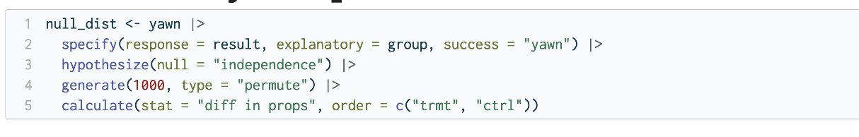
explain the steps for writing the code for simulation by computation

• start with the data frame

• specify the variables

• state the null hypothesis

• generate simulated differences via permutation

• calculate the sample statistic of interest

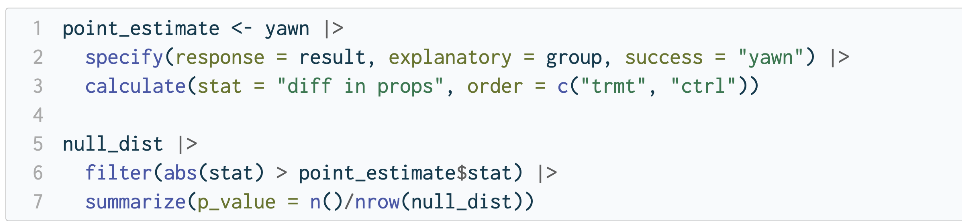
write the code for calculating the p value

significance level

the cutoff value for whether the p-value is low enough that the data are unlikely to have come from the null model

when is Ho rejected

if p-value < alpha, reject Ho in favour of Ha - the data provide convincing evidence for the alternative hypothesis

when is Ho not rejected

if p-value > alpha, fail to reject Ho in favour of Ha - the data do not provide convincing evidence for the alternative hypothesis

false positive

rejecting the null hypothesis when it is correct

false negative

failing to reject the null hypothesis when it is incorrect

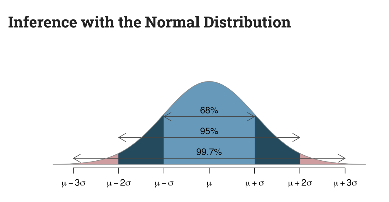
assumptions of the central limit theorem

• assumes sampling statistics adhere to a normal distribution

• observations in the sample are independent

• the sample size is sufficiently large

sketch the normal distribution curve

p-value

the probability of observing a test statistic as extreme as the one computed from the sample data, assuming the null hypothesis is true

why are permutation-based approaches used

they repeat simulations to estimate the distribution of the test statistic under the null hypothesis

code for generating the null distribution

set.seed(123)

what is the code for visualising a simulated p-value

visualize(null_dist) +
shade_p_value(obs_stat = d_hat, direction = "two-sided")

what is the code for calculating a simulated p-value

null_dist |>
get_p_value(obs_stat = d_hat, direction = "two-sided")

what function displays linear regression

fit()

statistical inference

the process of using sample data to make conclusions about the underlying population from which the sample came

estimation

uses data from samples to calculate sample statistics (mean, median, slope) which can then be used as estimates for population parameters

hypothesis testing

use data from samples to calculate p values which can then be used to evaluate competing claims about the population

confidence intervals

a plausible range of values for a population parameter; need to quantify the variability of the sample statistic in order to construct one

code for sampling without replacement

sample(x = 1:10, size = 10, replace = FALSE)

code for sampling with replacement

sample(x = 1:10, size = 10, replace = TRUE)

explain the bootstrapping scheme

1. take a bootstrap sample - a random sample taken with replacement from the original sample, of the same size as the original sample

2. calculate the bootstrap statistic - a statistic such as mean, median proportion, slope computed on the bootstrap samples

3. repeat steps 1 and 2 to create a bootstrap distribution

4. calculate the bounds of the confidence interval as the middle of the bootstrap distribution

code for taking a bootstrap sample

economy_boot_1 <- economy |>
slice_sample(n = nrow(economy), replace = TRUE)

explain the difference between confidence intervals and p values

• confidence interval: range of plausible values for the population parameter; distribution centred around the observed sample statistic

• p value: probability of observing the data, given the null hypothesis is true; distribution centred around the value from the null hypothesis

• a 95% confidence interval in practice is a hypothesis test with alpha = 0.05

code for calculating mean

calculate(stat = “mean”)

code for obtaining the confidence interval

get_ci(x = boot_df, level = 0.95)

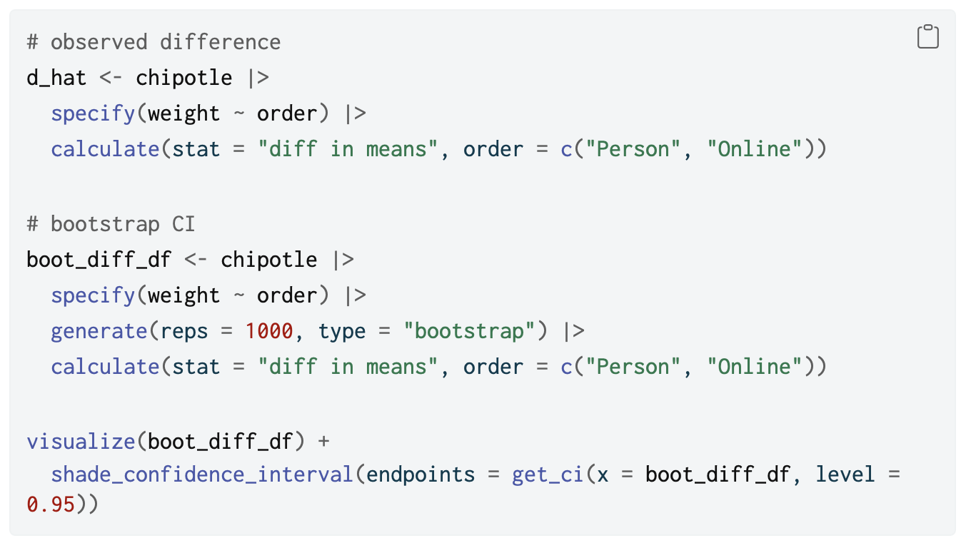
entire code for the chipotle confidence interval problem

modeling

the use of models to explain the relationship between variables and to make predictions

linear models

classic forms used for statistical inference

nonlinear models

much more common in machine learning for prediction

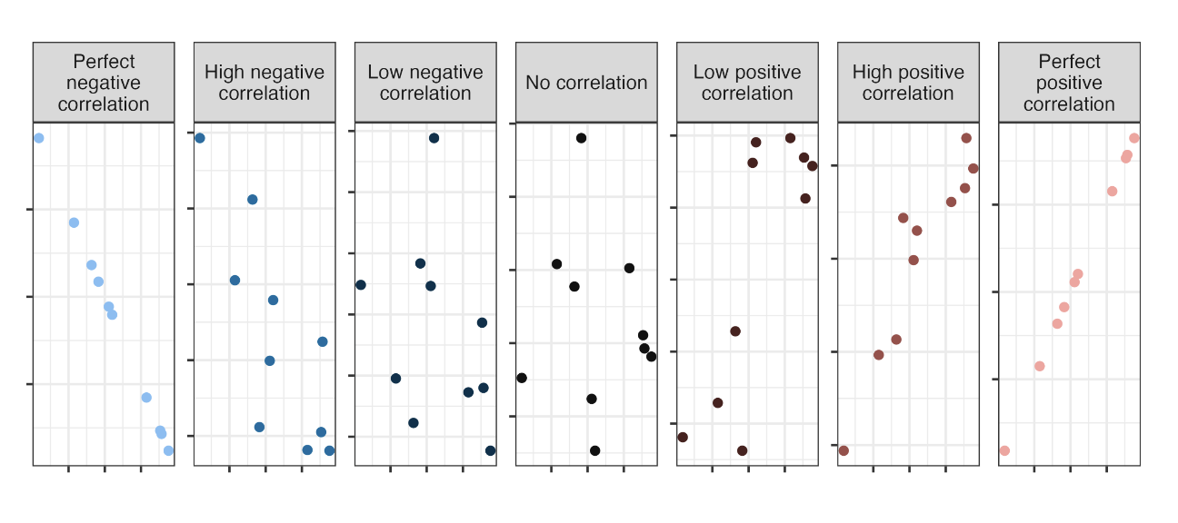
correlation

ranges between -1 and 1, same sign as the slope

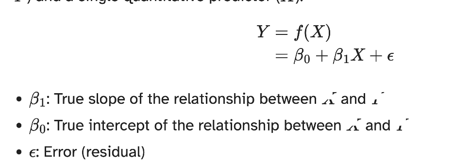
regression model

a function that describes the relationship between the outcome and the predictor; Y =Model + Error

simple linear regression

used to model the relationship between a quantitative outcome and a single quantitative predictor

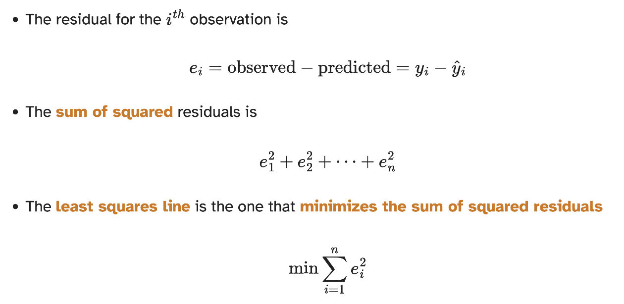
residual formula

observed - predicted

least square lines

minimises the sum of squared residuals

code for simple linear regression

movies_fit <- linear_reg() |>
fit(audience ~ critics, data = movie_scores)

tidy(movies_fit)

properties of least squares regression

• The regression line goes through the center of mass point (the coordinates corresponding to average x and y coordinates)

• Slope has the same sign as the correlation coefficient

• Sum of the residuals is zero

• Residuals and values are uncorrelated

in what context is the intercept meaningful

when the predictor has values near zero