Intermediate Micro

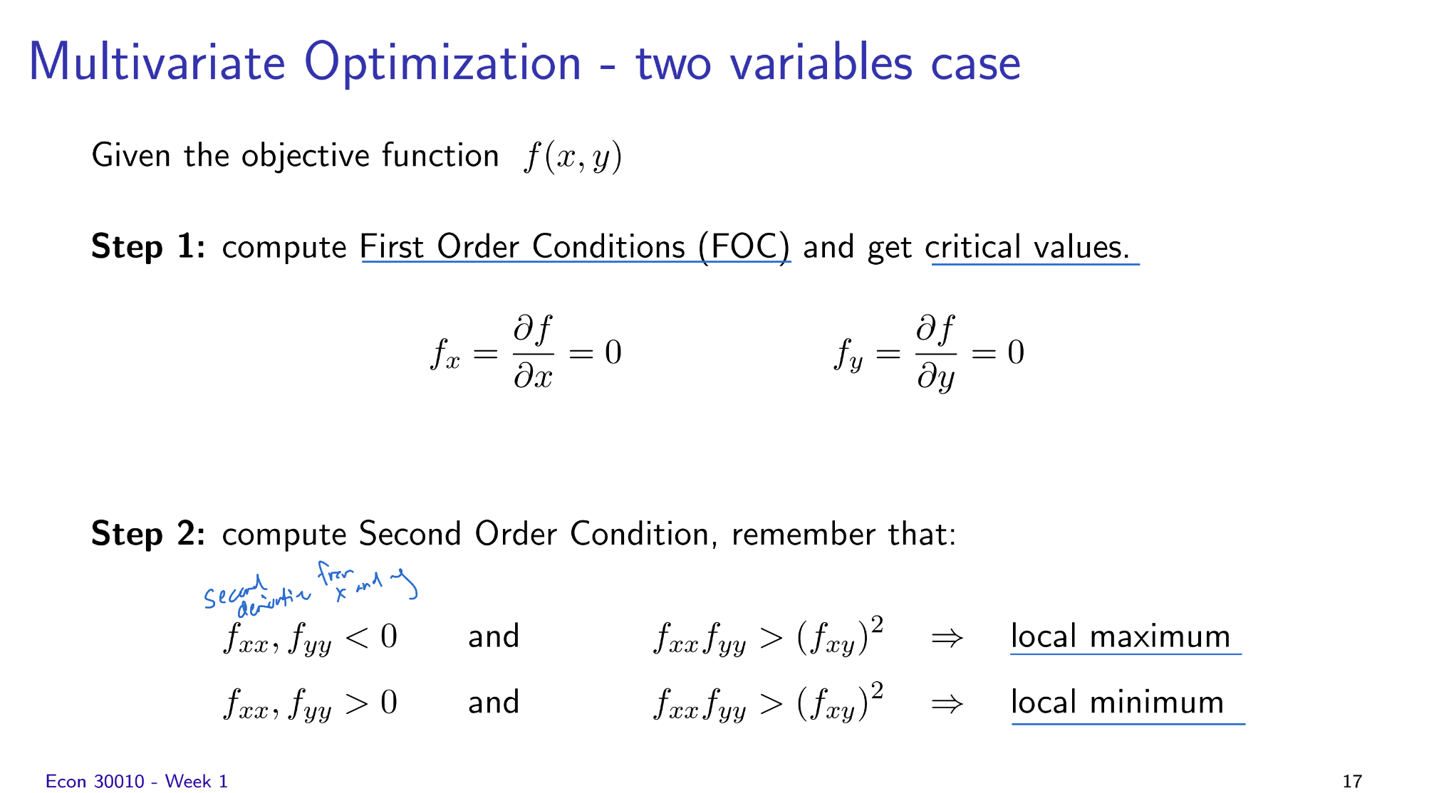
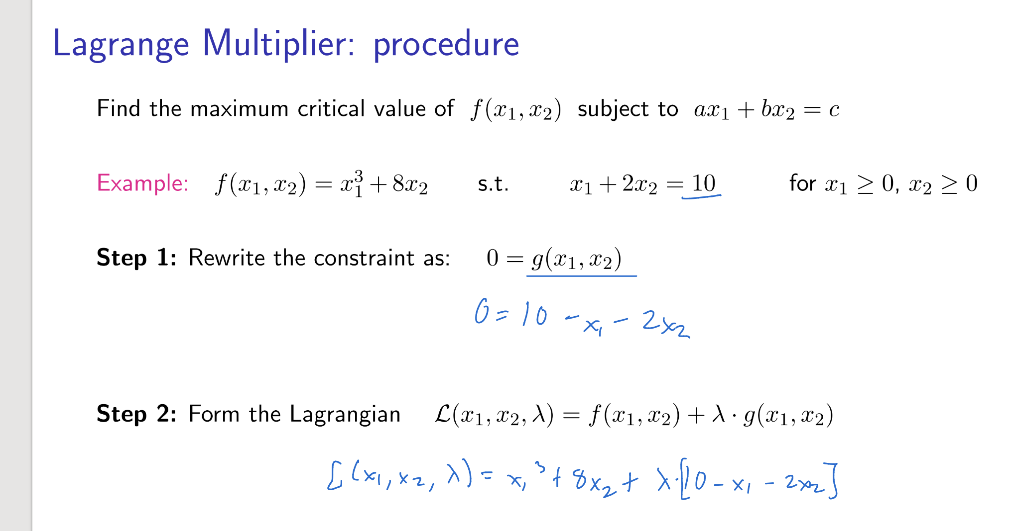
Multivariable Optimization

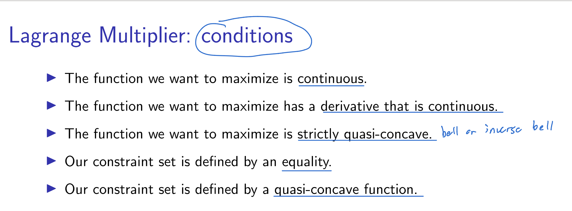
Larange Multiplier Conditions

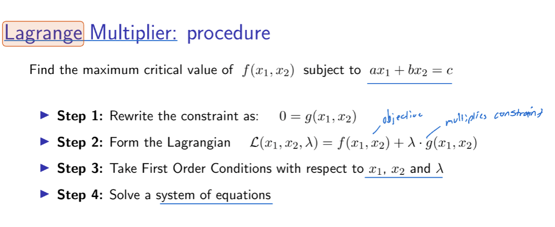
Larange Multiplier Procedure

example:

Preference Outlines

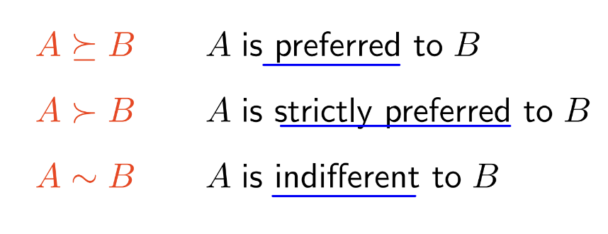
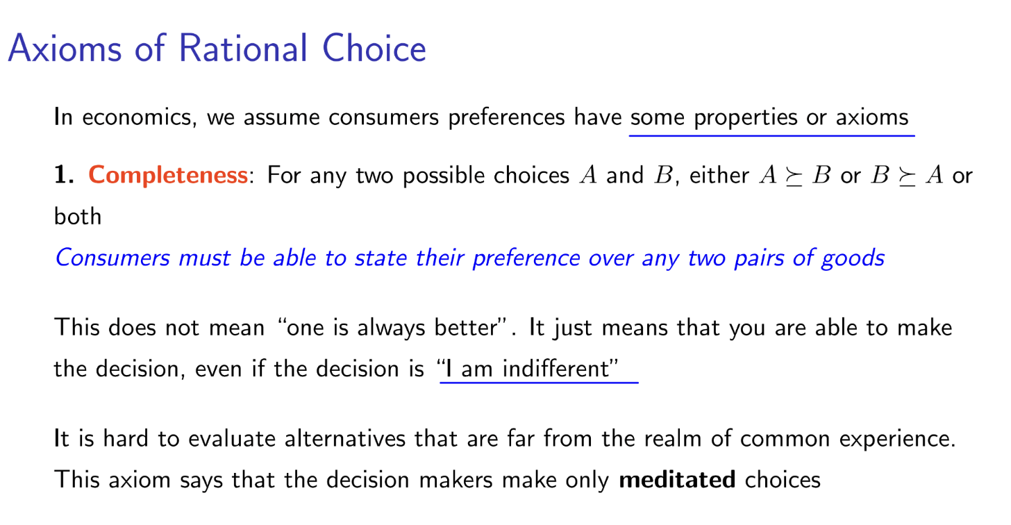
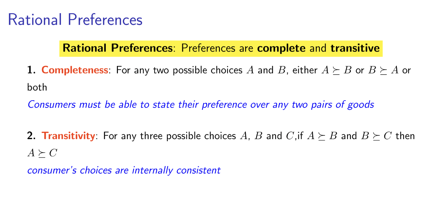
Completeness

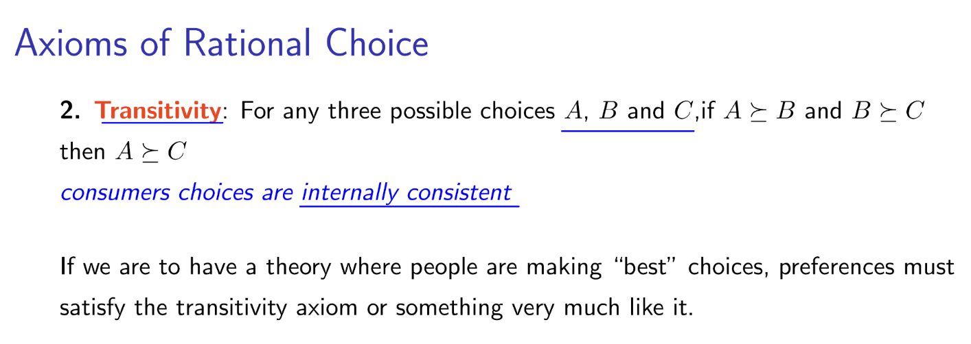
Transitivity

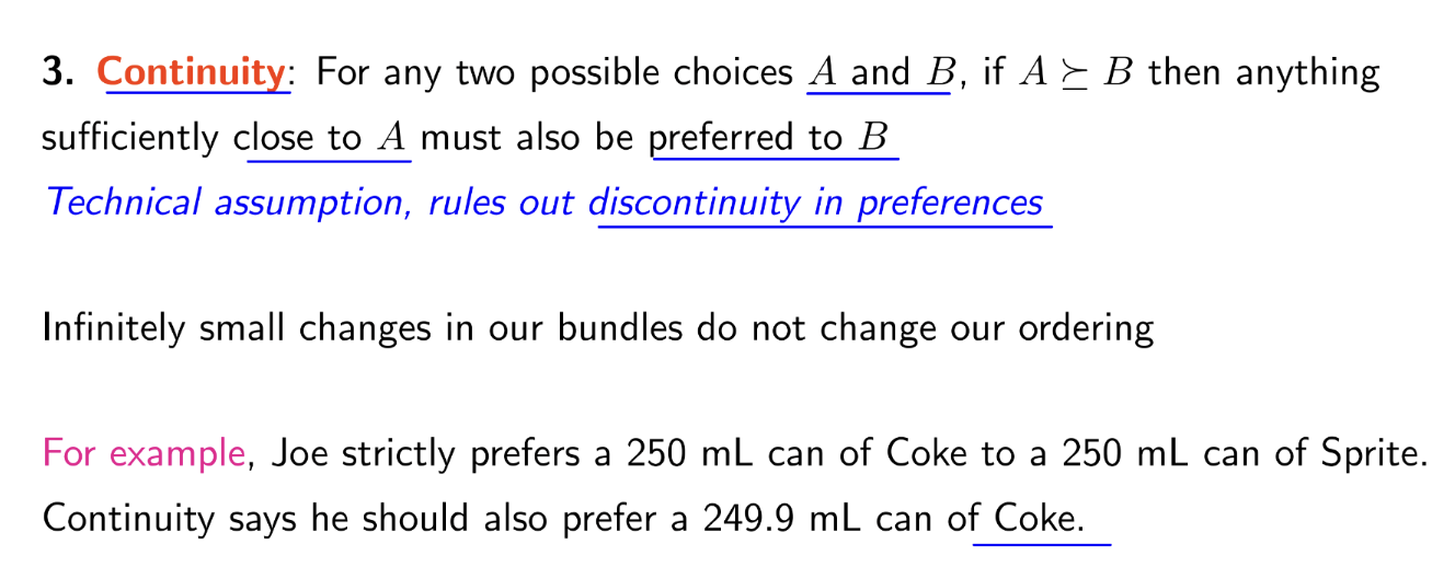
Continuity

Monotonicity

A preference relation displays monotonicity if, for each bundle, A, every bundle, B, with more of each good in the bundle is strictly preferred.

Strong monotonicity

A preference relation displays strong monotonicity if, for each bundle, A, every bundle, B, with the same amount of each good and more of at least one good in the bundle, is strictly preferred

example:

The Rule: "More of any good is strictly better."

• Simple Example:

  • Bundle A: (2 Pizzas, 1 Soda)

  • Bundle B: (2 Pizzas, 2 Sodas)

    • Under Strong Monotonicity, Bundle B is strictly preferred to Bundle A because it has more soda and no less pizza.

Rational Preferences

Preferences are complete and transitive

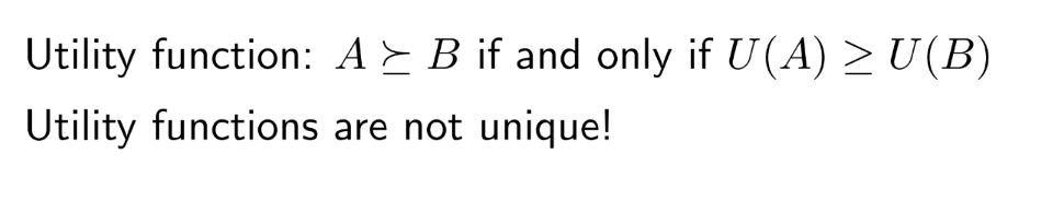
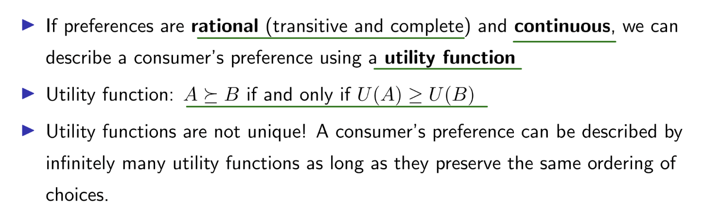
Utility Functions

Indifference map

complete set of indifference cures that summarize a consumer’s tastes

Indifferences curves with rational and monotonic preferences must b

1. non-increasing

2. “thin”

3. non-crossing (due to monotonicity and transitivity)

4. preferred as they move farther from the origin

5. convex

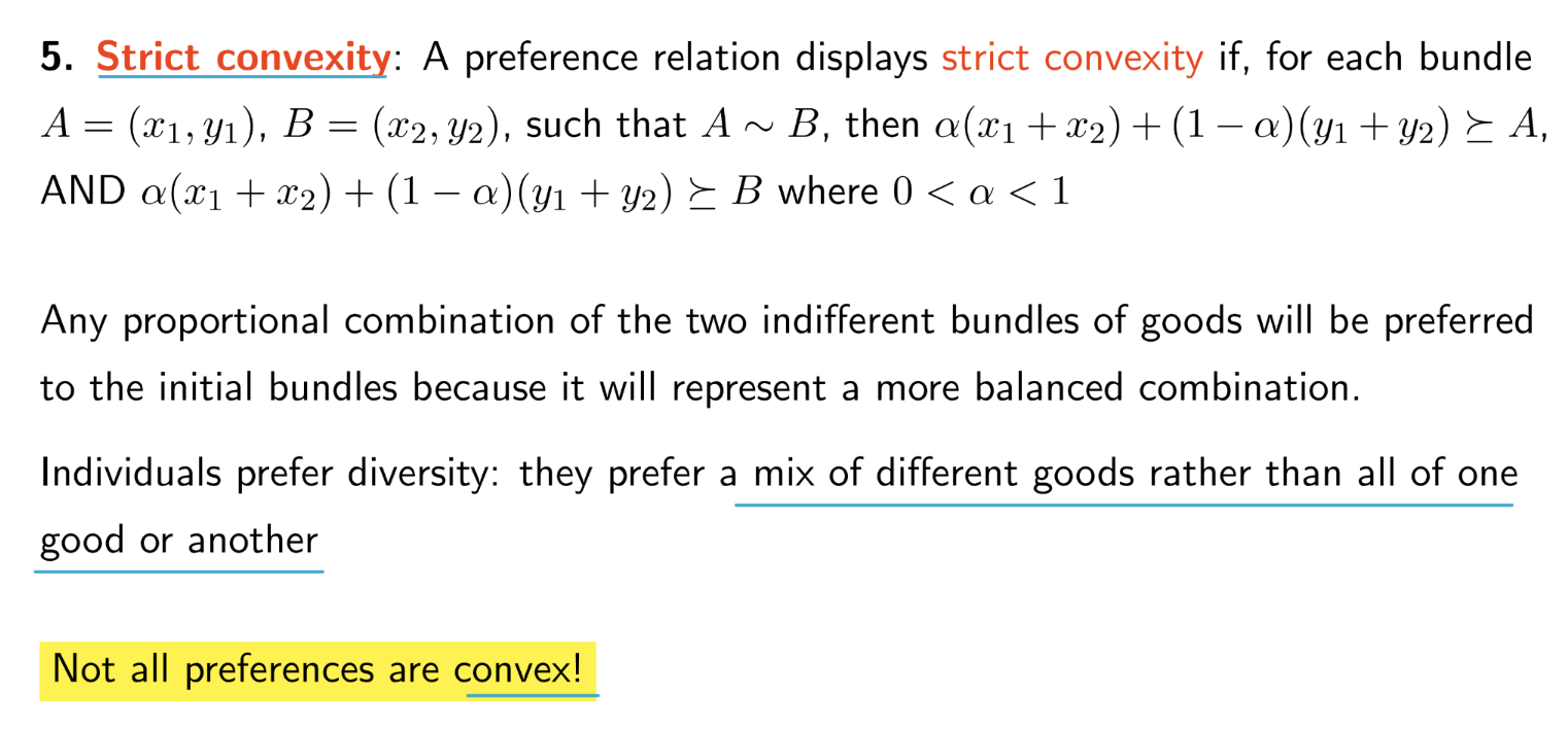
Strict convexity

example : A consumer with convex preferences is indifferent between 2 hamburgers or 4 slices of pizza. Given their preferences we know (2h, 0p) indifferent (0p, 4p)

lets define A=(2,0) and B=(0,4)

convexity tells us that they would prefer a mix of hamburgers and pizza rather than all of one good or another. → Any combination of these 2 bundles would be preferred

For example, we can create a combination using half of each bundle:

1/2(A)+1/2(B) = (1/2(2)+1/2(0), 1/2(0)+1/2(4)) = (1,2)

They prefer 1 hamburger and 2 slices of pizza to either of A or B.convex

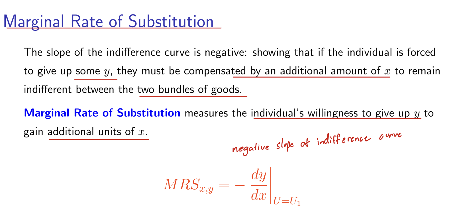
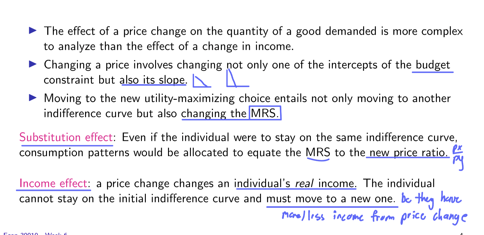
Marginal Rate of Substitution

Measures the individual’s willingness to give up y to gain additional units of x.

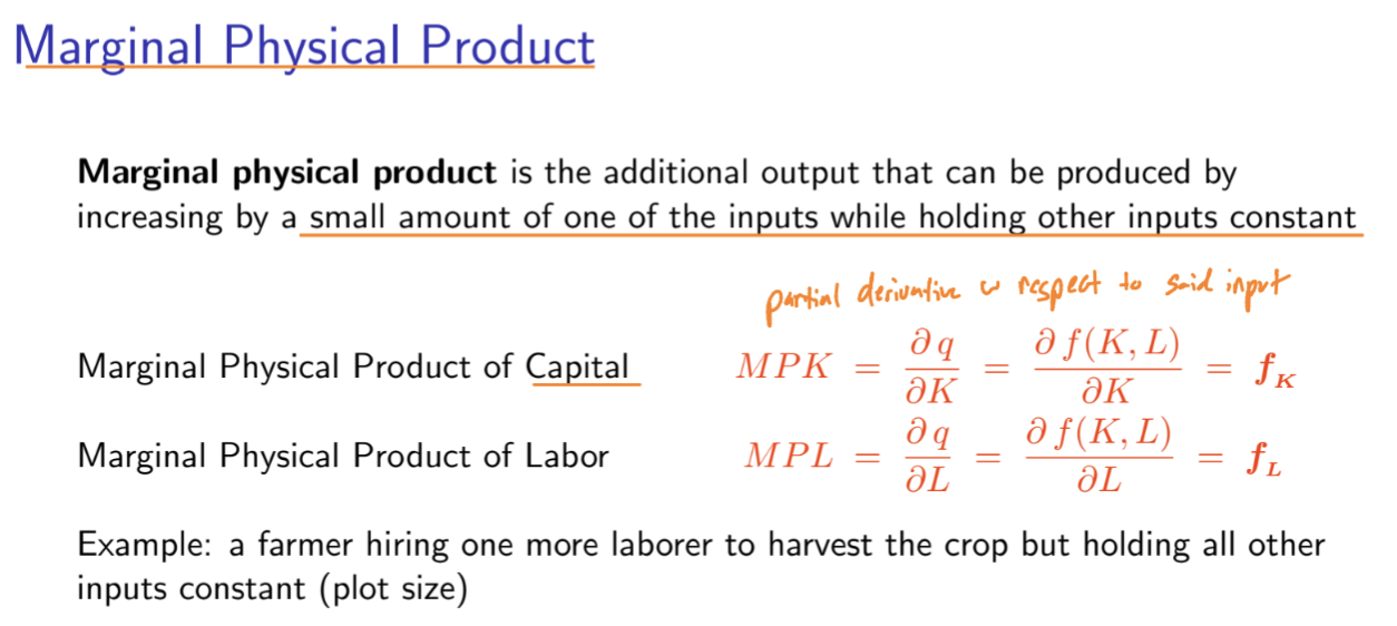
Marginal Utility

How much additional utility an individual receives from consuming one more unit of x (or y)

Ux= du(x,y)/dx and Uy= du(x,y)/dy

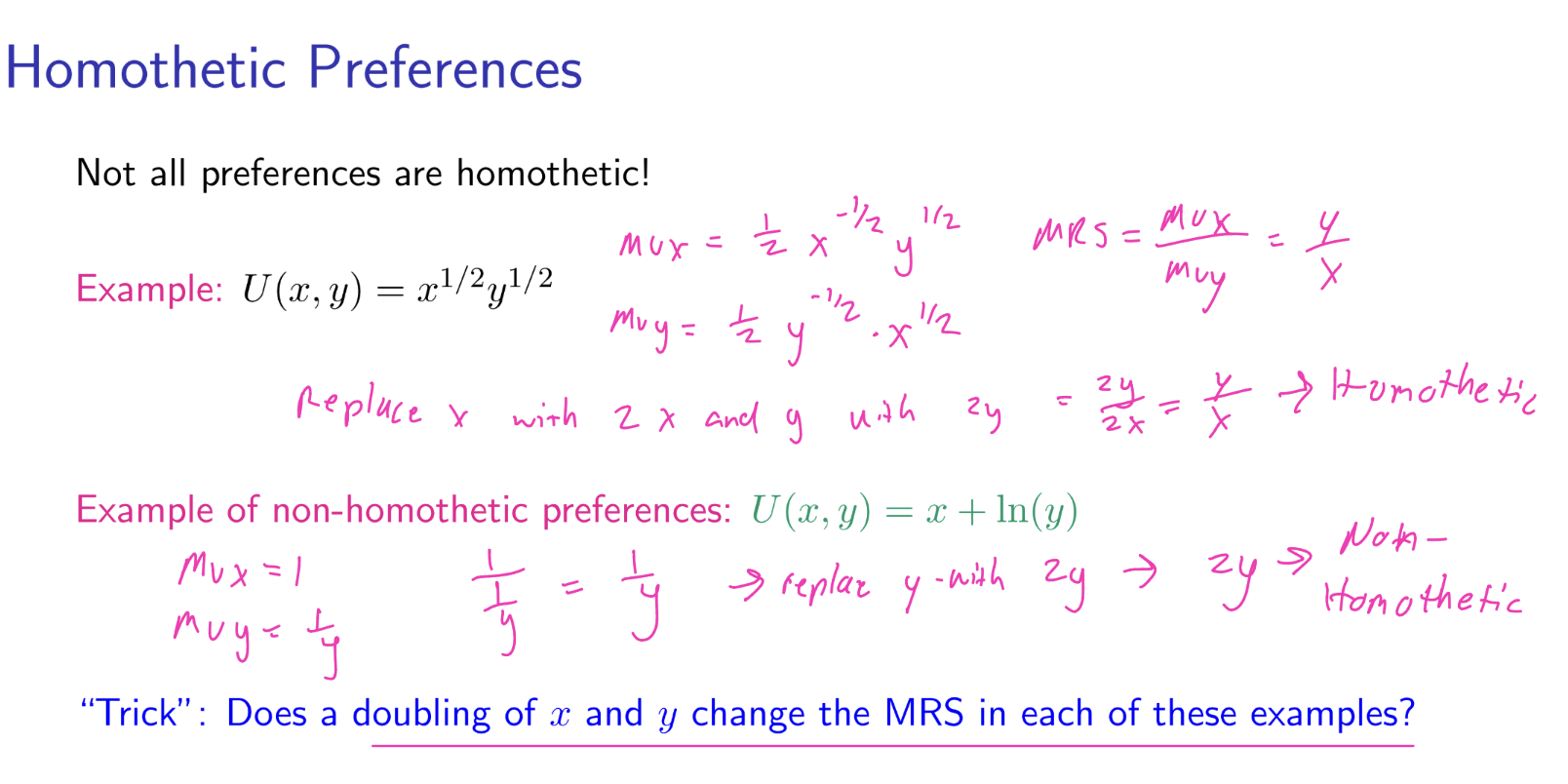
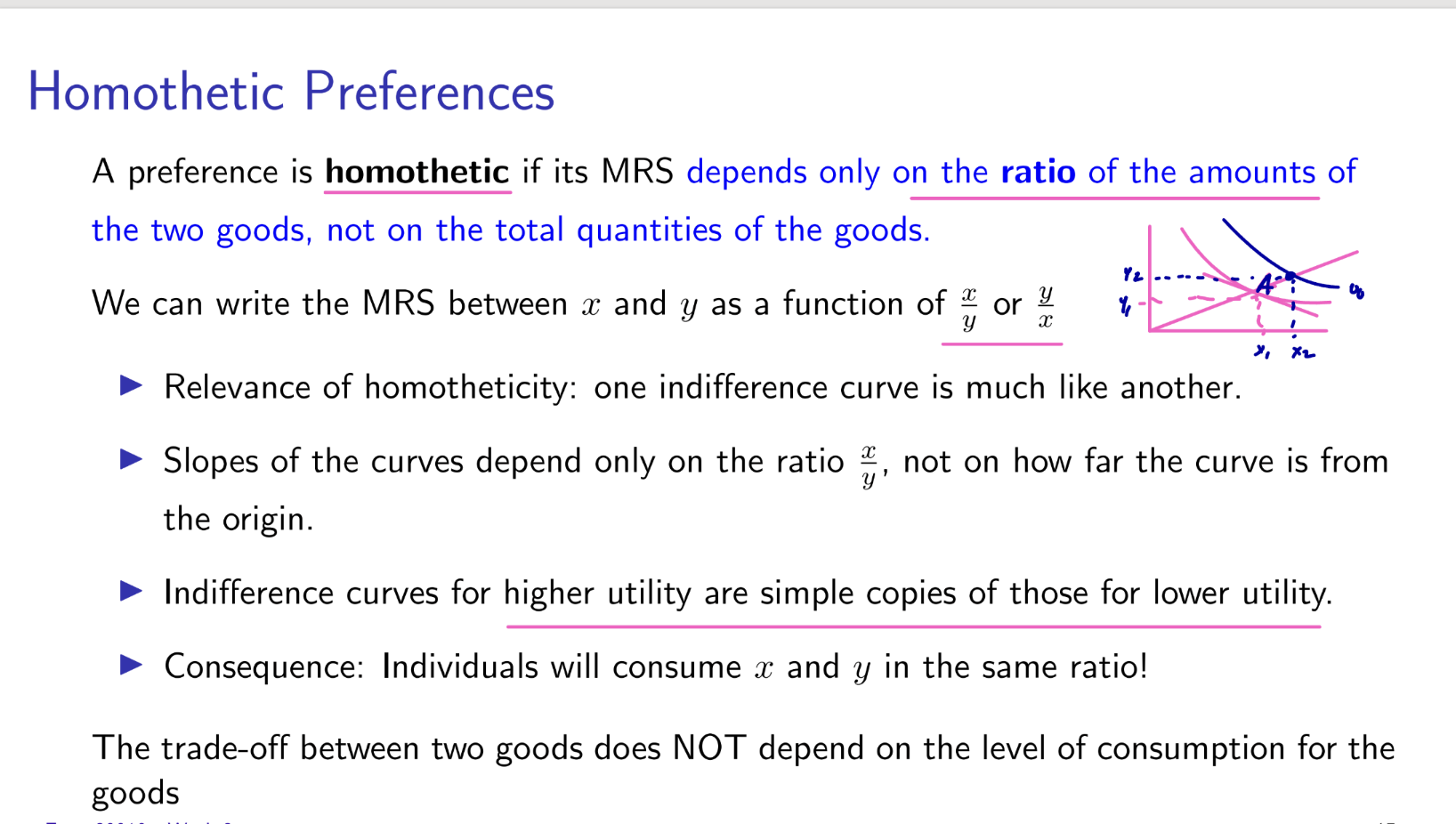
Homothetic Preferences

example:

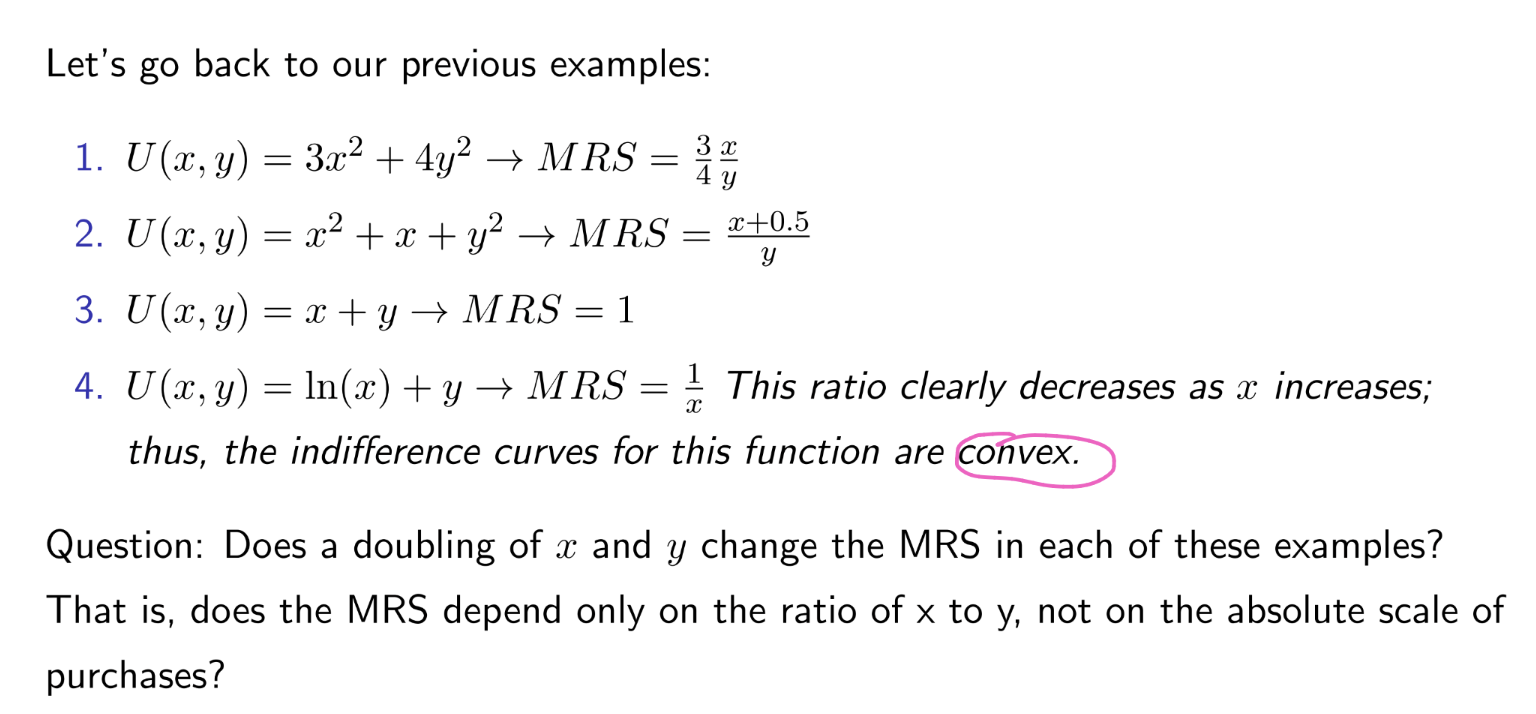
Showing Convexity of Indifference Curves

To check for convexity we see how MRS changes along an indifference curve. For convex preferences, MRS is decreasing in x.

dMRS(x,y)/dx < 0

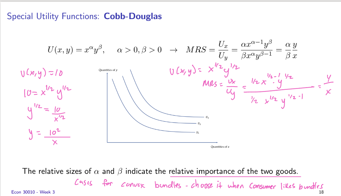
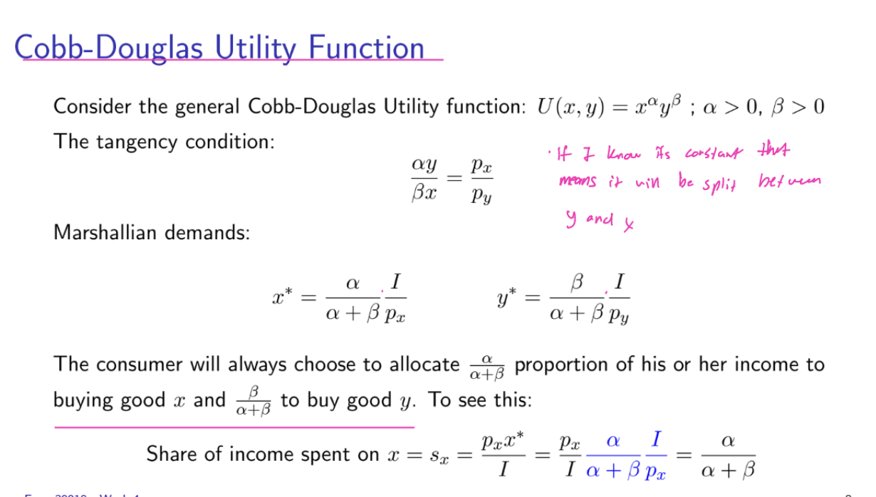
Special Utility Functions : Cobb-Douglas

Essentially a shortcut in finding MRS for functions that have a U(x,y)= x^A* y^B

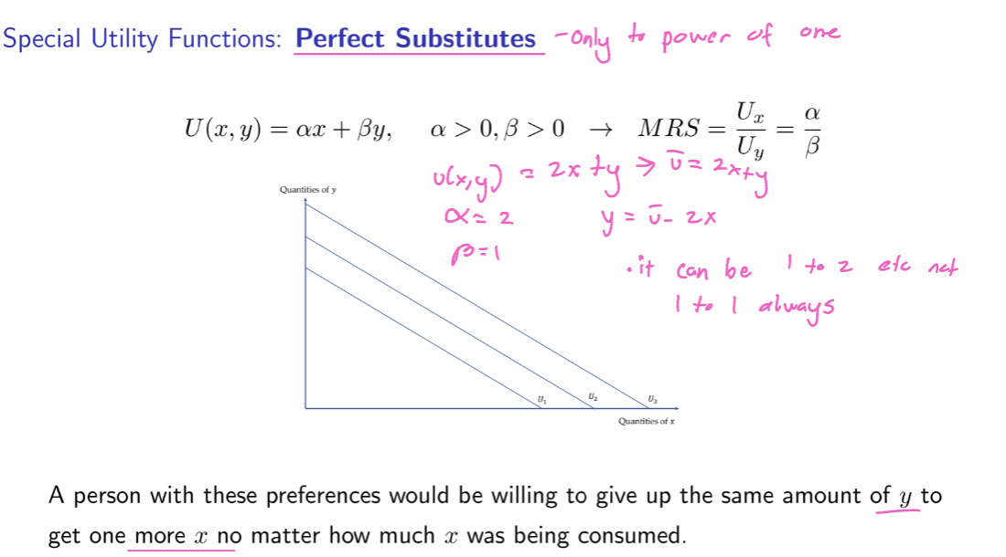
Special Utility Functions: Perfect Substitutes

only to the power of one

Functions of utility that look like

U(x, y) = ax+ by. a>0, b>0 and MRS = Ux/Uy = a/b

Two goods are perfect substitutes if the consumer doesn't care about the brand or source, only the total amount. They are willing to trade one for the other at a constant rate(which hints at the straight lines for their utility)

The Key: If the problem says "the consumer is always willing to trade 1 unit of X for 2 units of Y," you are looking at perfect substitutes.

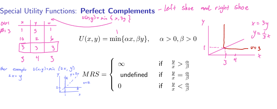
Special Utility Functions: Perfect Complements

In these problems, having more of one good is useless unless you get more of the other. They are consumed together in specific proportions.

• Example: You are building bicycles. You need exactly 2 tires (x1) and 1 frame (x2). Having 10 tires and only 1 frame still only gets you one finished bike.

• The Key: Look for phrases like "always used together," "required in a ratio of," or "cannot use one without the other."

  • Why "Min"? Because your utility is limited by the "minimum" amount of a pair you have. If U = min{x1, x₂} and you have 10 of x1 but only 1 of x2, your utility is min{10, 1} = 1. The extra 9 units of x1 are "wasted."

The Vertex: The "kink" or corner of the L-shape occurs exactly where ax1 = bx2.

The MRS: This is the math "gotcha." At the corner, the derivative is undefined.

• On the horizontal part of the "L", the MRS = 0.

• On the vertical part of the "L", the MRS = infinity.

The Budget Constraint

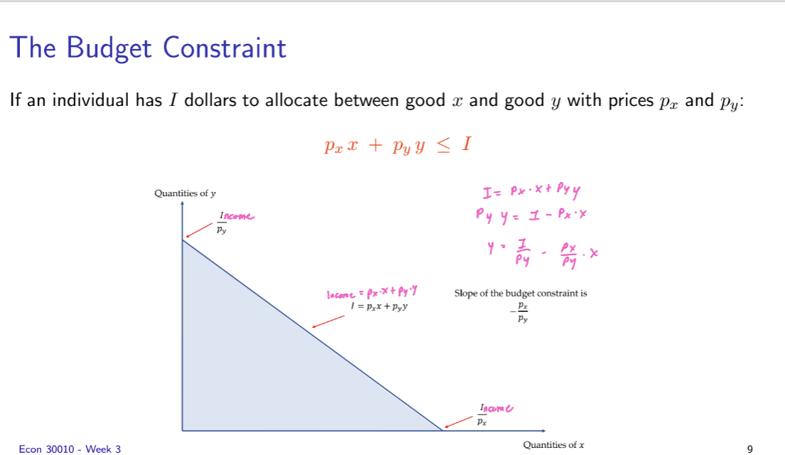
monotonicity assumption

implues that the individual should spend all of his or her income to receieve maximum utility

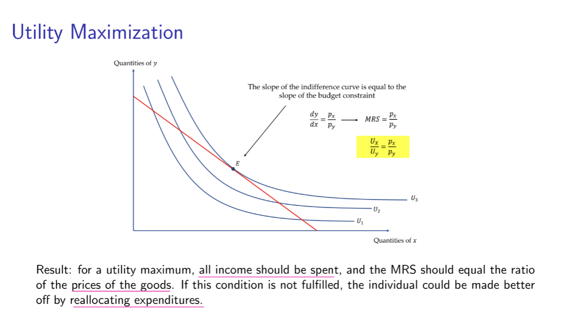
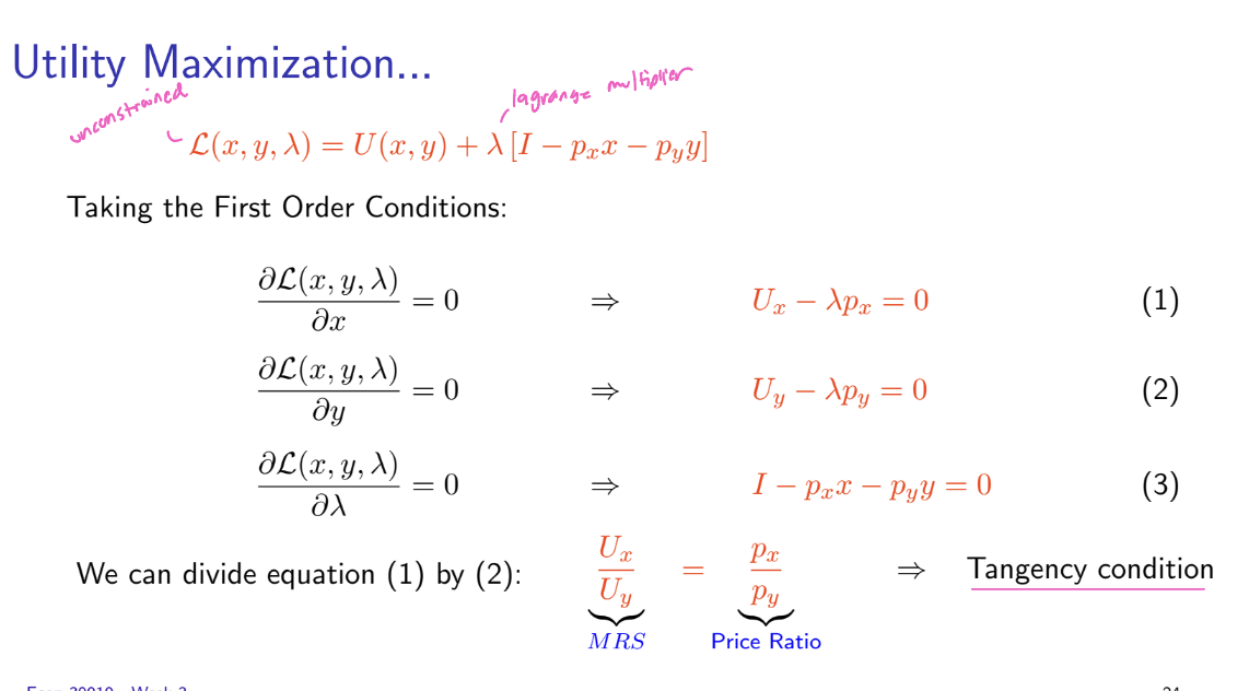
Conditions for Utility Maximization

For a utility maximum, all income should be spent, and the MRS should equal the ratio of the prices of the goods. If this condition is not fulfilled, the individual could be made better off by reallocating expenditures.

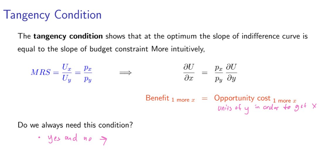
Tangency Condition

• The tangency condition is only necessary but not sufficient unless we assume that MRS is diminishing

• If MRS is diminishing, then indifference curves are strictly convex and we always have a maximum where MRS = px/py

• If MRS is not diminishing, then we should check second-order conditions to ensure that we are at a maximum

• essentially, it is setting our MRS = px/py

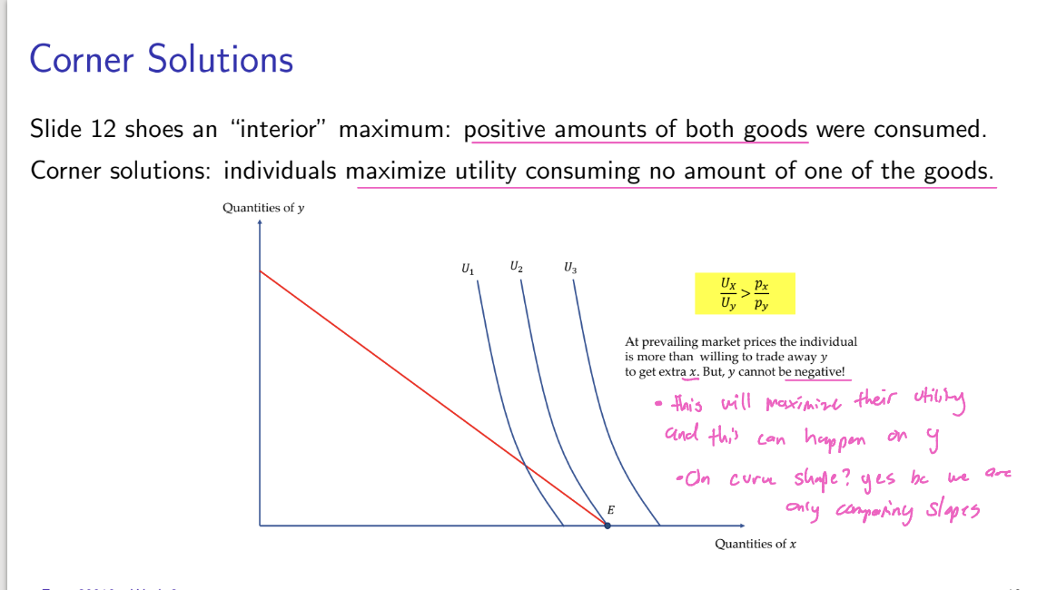
“interior” maximum

positive amounts of both goods were consumed

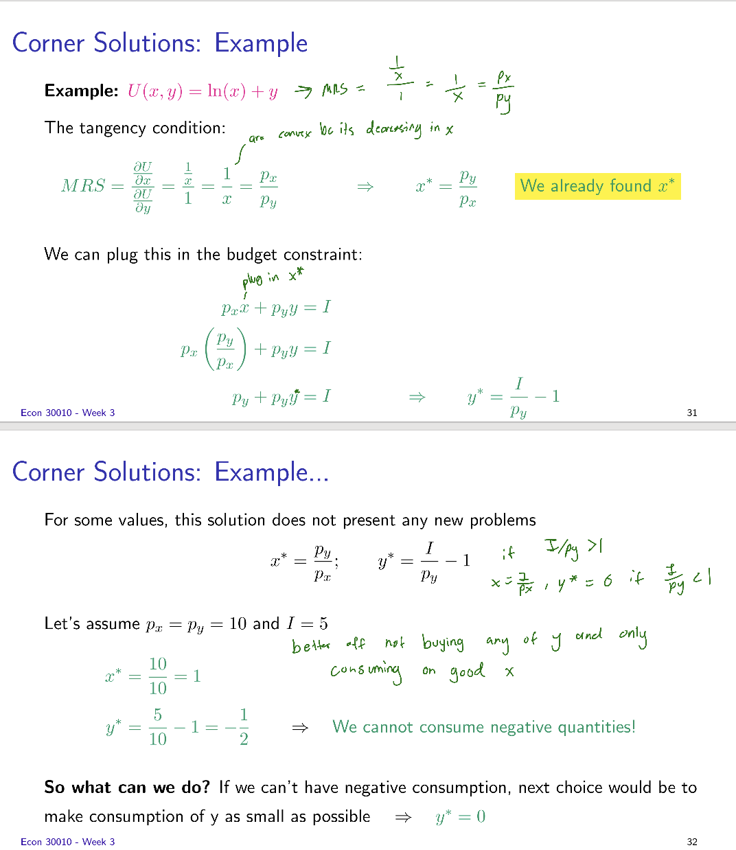
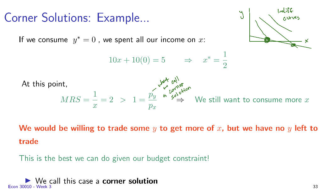
Corner solutions

individuals maximize utility consuming no amount of one of the goods

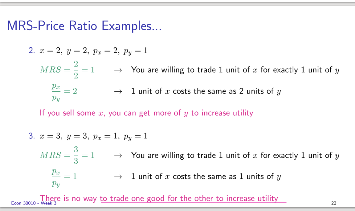
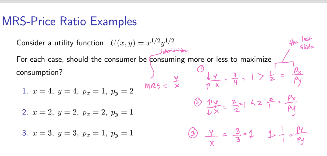
MRS- Price Ratio Examples

More examples:

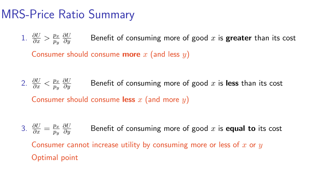
MRS - Price Ratio Summary

Lagrange and MRS | Price Ratio

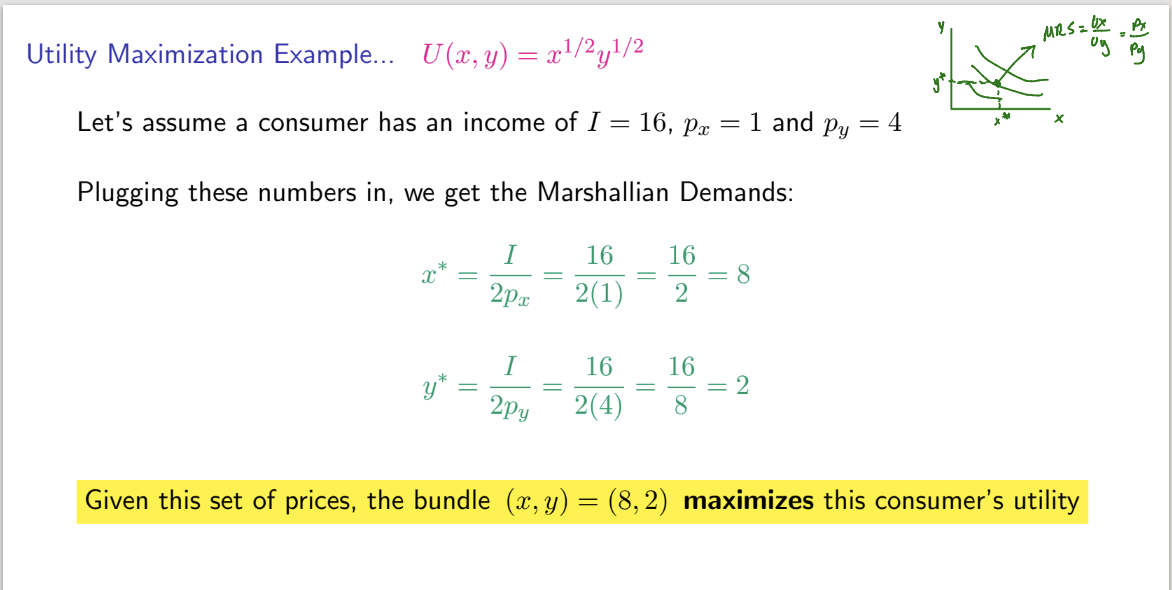
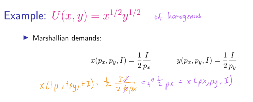
Marshallian Demands

Using the tangency condition, we solve for the optimal choices of x and y as functions of the prices and income (using the Lagrange function, then put (dL/dx)/(dL/dy))=y/x and solve for one variable ex y and then use that to plug into our original px*x+py*y=I function to solve for y* and x*.

x* = x(px,py,I) = gx(px,py,I)

y* = x(px,py,I) = gy(px,py,I)

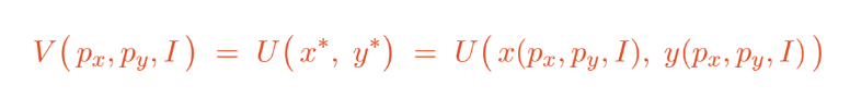
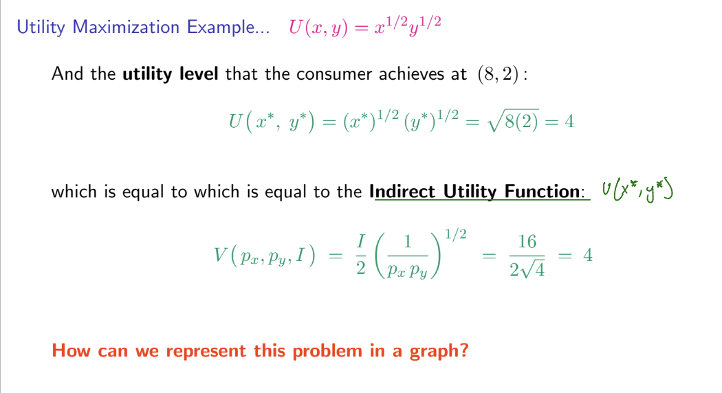
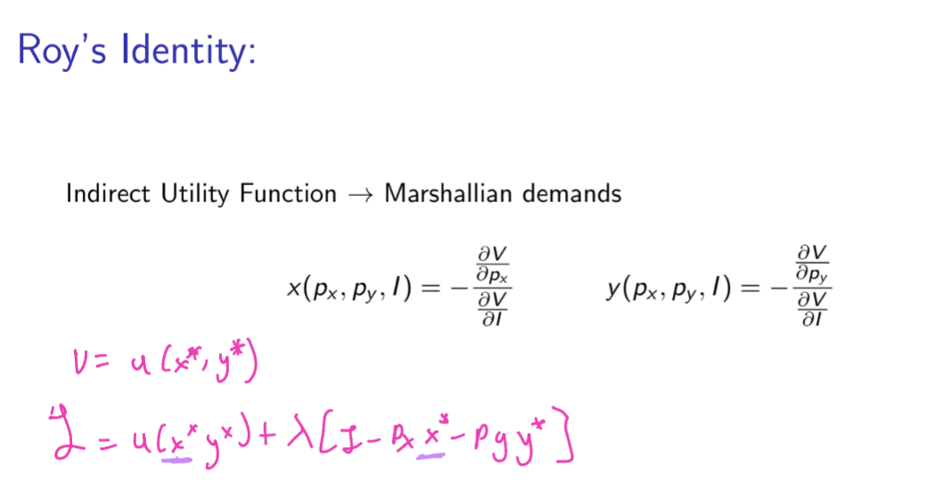
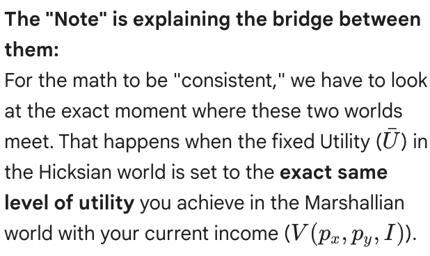
Indirect Utility Function

Using the X* and Y* we got from solving for marshallian Demands, we plug them into our utility function and then we obtain our indirect utility function that only depends on the prices and income

Utility Maximization Bundle and Utility Solving

Corner Solutions Example

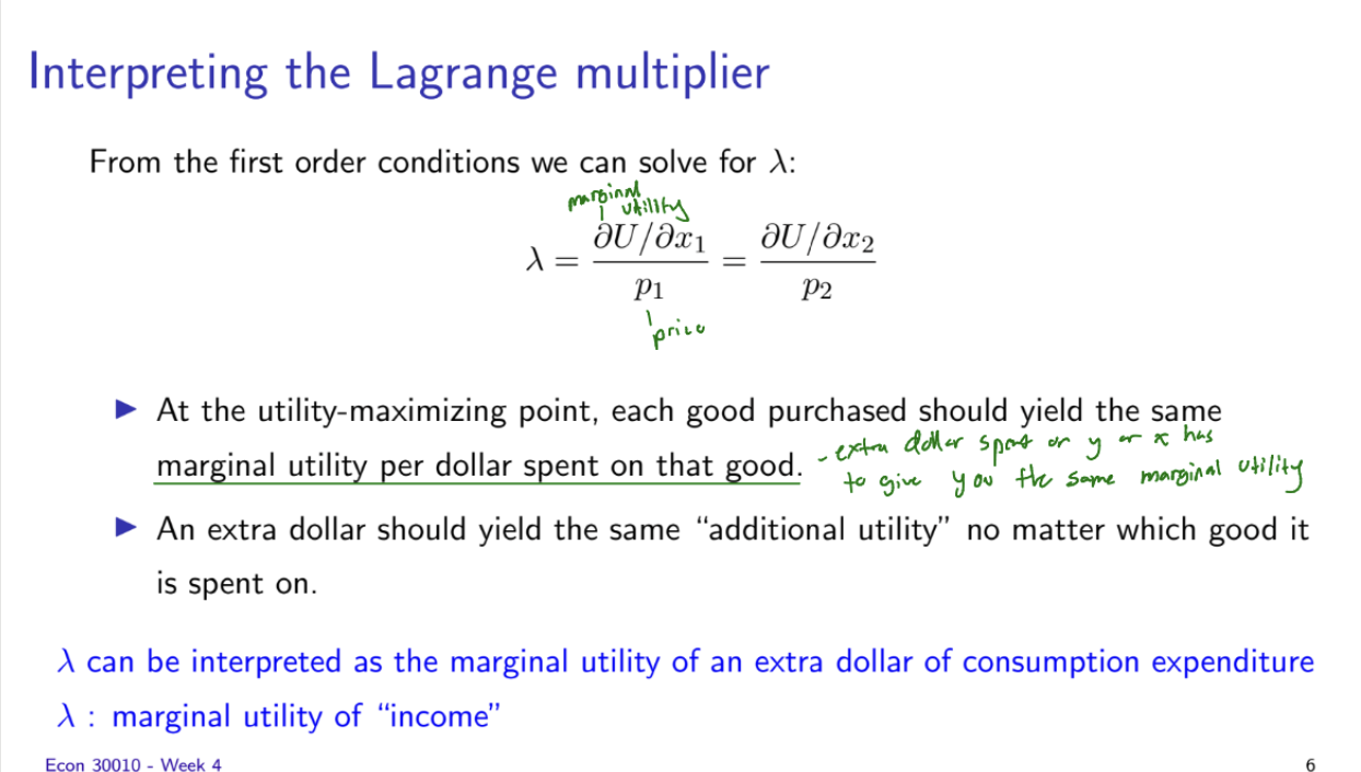
Interpreting the Larange Multiplier

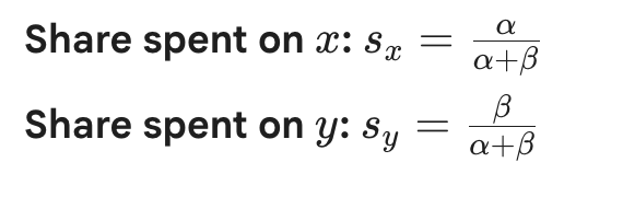
Cobb-Douglas Demand Shortcut

Goal: Find the optimal x^a and y^b without using a Lagrangian

To make this flashcard-ready, let’s strip away the fluff and focus on the "plug-and-play" logic. You want the Standard Form, the Shortcut, and the Intuition.

---

Flashcard Front: Cobb-Douglas Demand Shortcut

Utility Function: $U(x, y) = x^{\alpha} y^{\beta}$

Goal: Find the optimal $x^*$ and $y^*$ without using a Lagrangian.

---

Flashcard Back: The "Income Share" Rule

1. The Logical Rule

The consumer always spends a fixed percentage of their income (I) on each good, regardless of prices.

2. The Demand Formulas (Marshallian Demand)

To find the quantity, take the money allocated to that good and divide by its price:

$$x^* = \left( \frac{\alpha}{\alpha + \beta} \right) \frac{I}{p_x}$$

$$y^* = \left( \frac{\beta}{\alpha + \beta} \right) \frac{I}{p_y}$$

3. Quick Example

If U = x^3 y^2:

• Total "parts": $3 + 2 = 5$

• Spend on x: 3/5 (or 60%) of income.

• Spend on y: 2/5 (or 40%) of income.

---

Expenditure Minimization

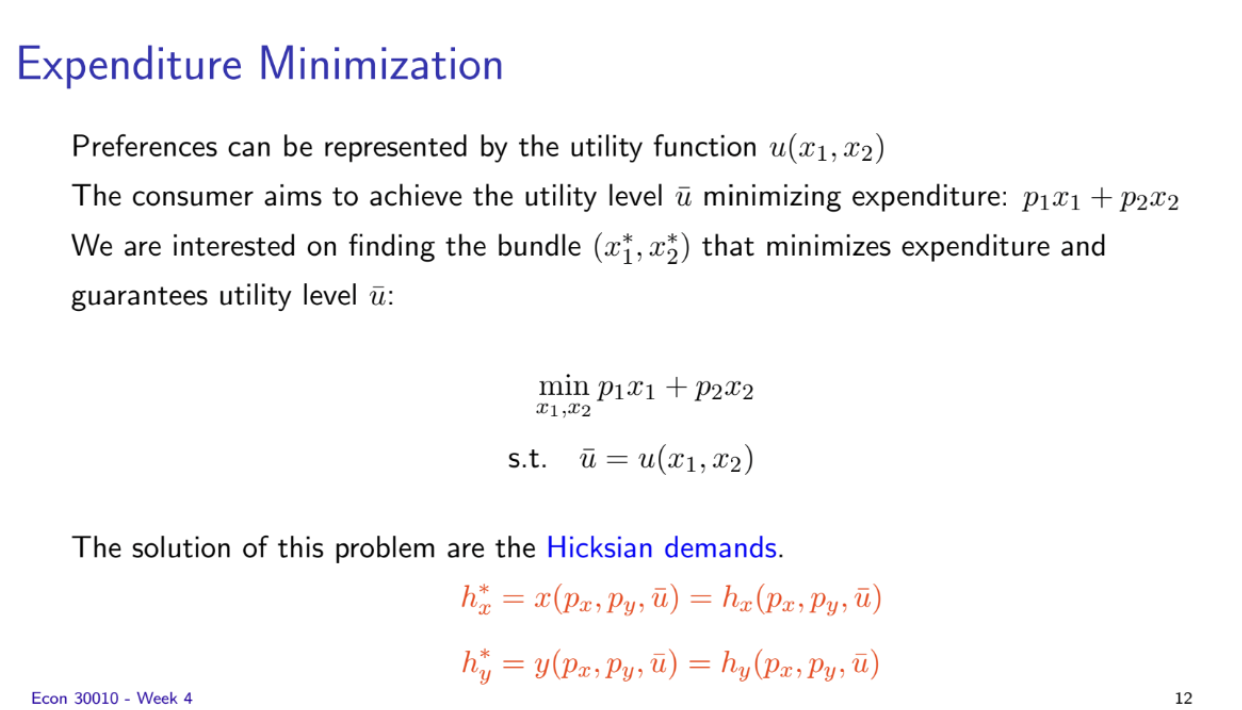
Hicksian Demand

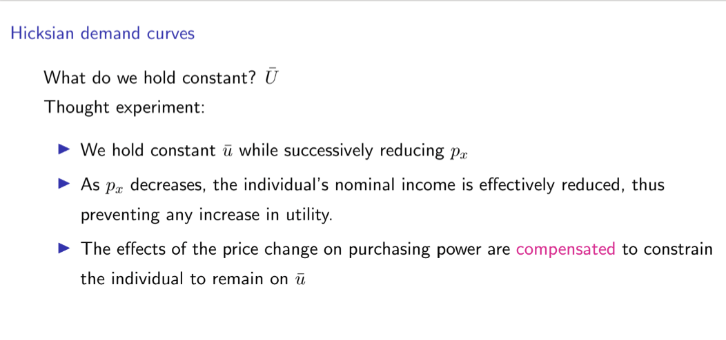
Hicksian demand asks, "Given a target utility, what is the cheapest way to get there?"

1. The Math Signature

Hicksian demand functions are written as hx (px, py, U).

• Note: They depend on Utility (U), NOT Income (I).

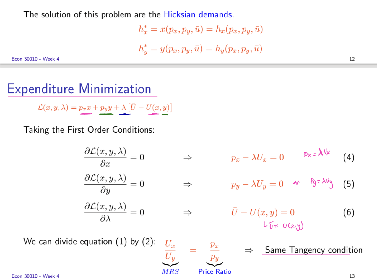
2. How to Solve (3 Steps)

1. Tangency: Set MRS = (p/x)/(py) (This is the same as Marshallian!).

2. Substitute: Solve for one variable (e.g., y = {something} * x).

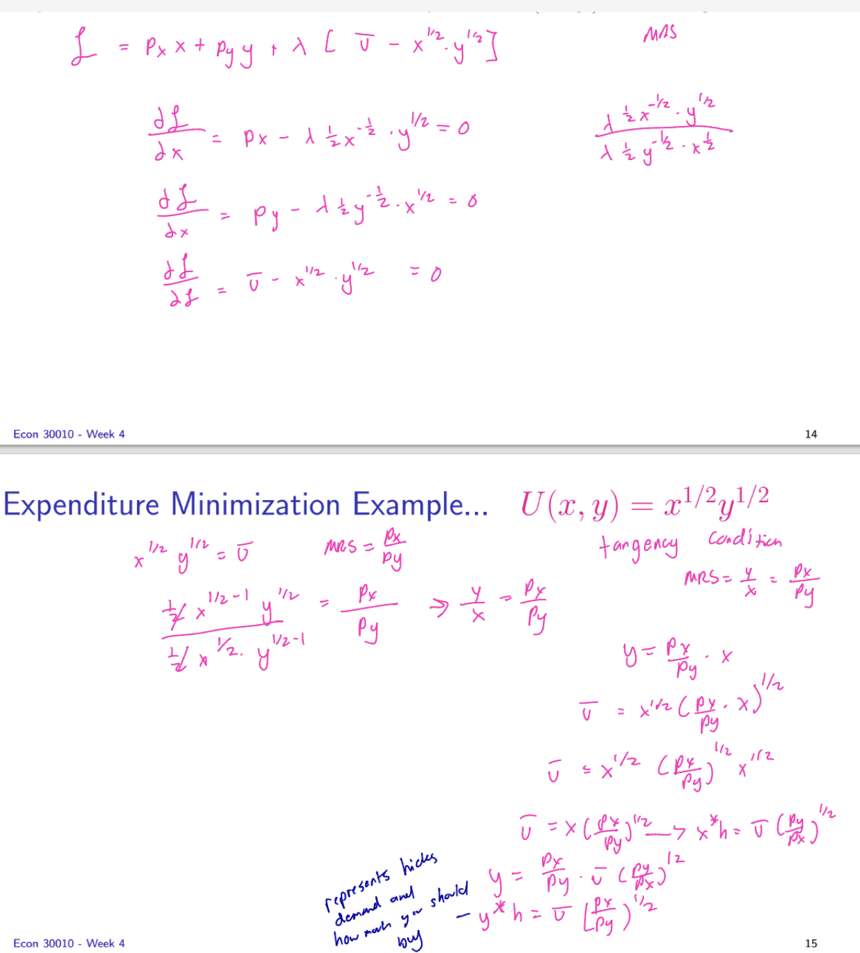
3. The Utility Constraint: Plug that into the Utility Function (not the budget line):

   $$\bar{U} = x^\alpha ( \text{your substitution for } y )^\beta$$

4. Isolate x: Solve for x to get x^h.

5. to solve for y*h then you use the x^h and plug it back in for your function of y= (somethig)*

The "Why" (Pro-Tip for Exams)

Hicksian demand is often called "Compensated Demand." If the price of x goes up, Hicksian demand assumes someone gives you just enough extra cash to stay on your original indifference curve. This is why it "isolates" the substitution effect—it removes the "I feel poorer" (income) effect entirely.

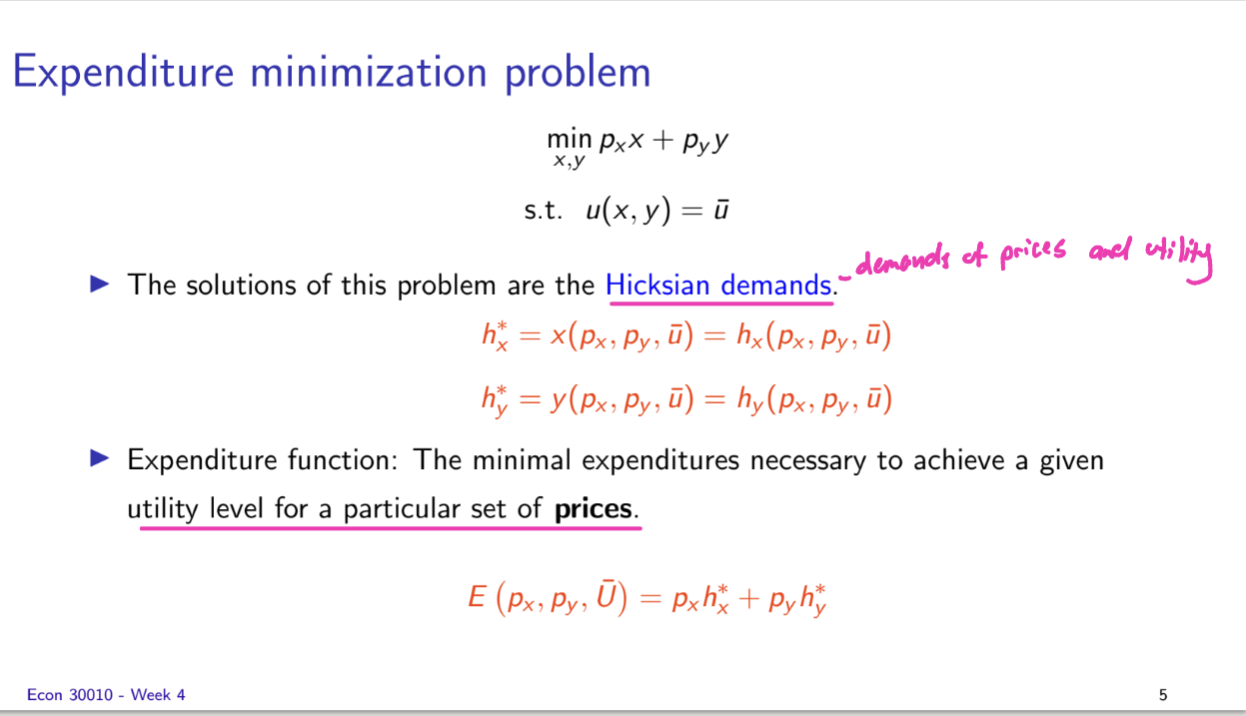
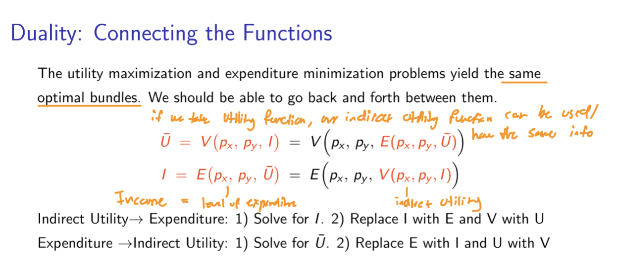
Expenditure Function

The individual’s expenditure function shows the minimal expenditures necessary to achieve a given utility level for a particular set of prices. That is E(p1, p2, ……pn, U)

The expenditure and the indirect utility function are inverse functions of one another.

Homogenous Functions - Definition

Expenditure minimization

Properties of the expenditure function

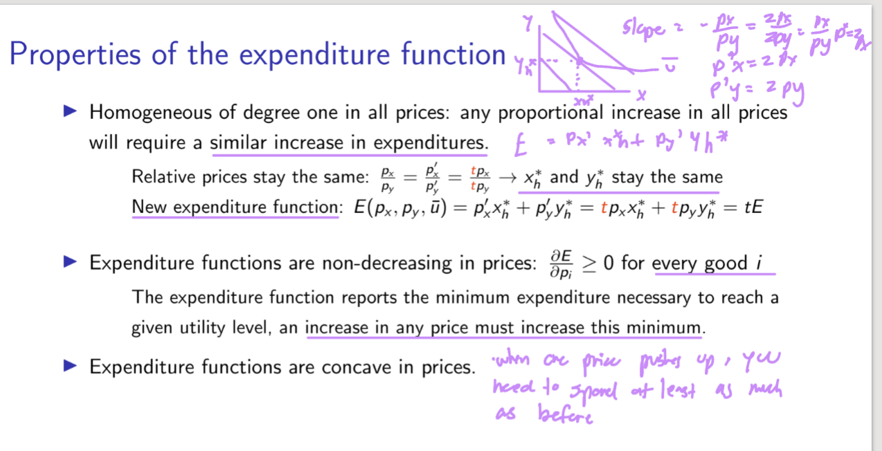
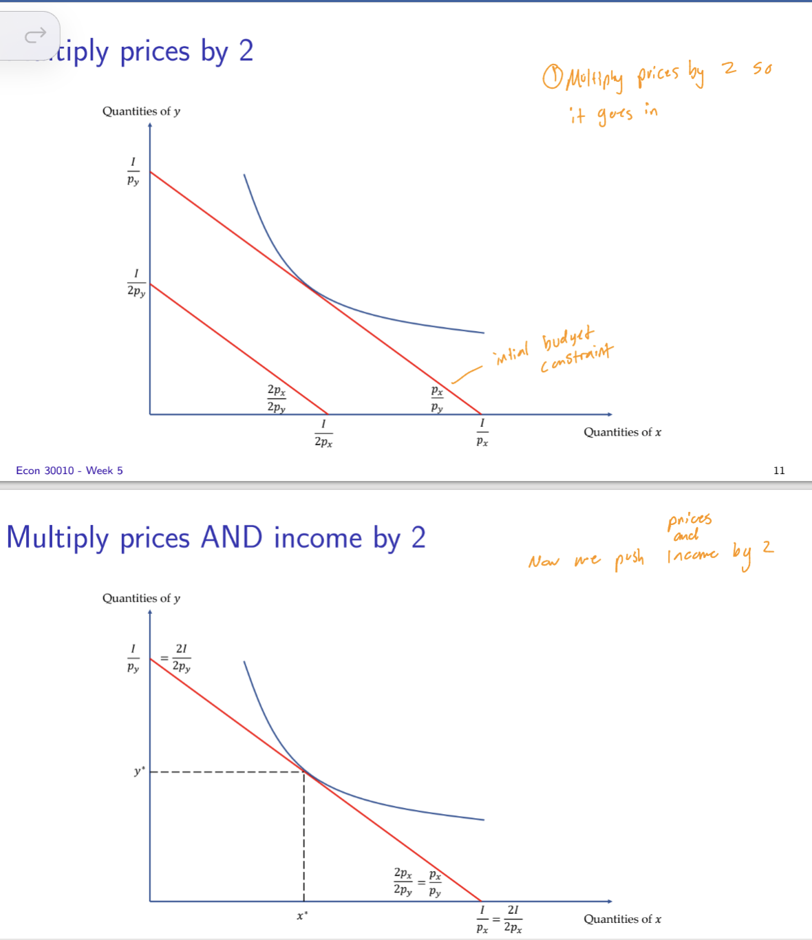
1. HD1 (The "Double Everything" Rule)

If you multiply all prices by a constant (t), your total expenditure must increase by that same constant (t).

• Logic: Doubling prices doubles your bill because the relative prices stay the same, so you don't change your behavior.

2. Non-Decreasing (The "More Expensive" Rule)

If any price (pi) goes up, your minimum spending (E) must go up or stay the same.

• Logic: You can’t stay just as happy for less money when things cost more.

3. Concave (The "Substitution" Rule)

The function grows at a decreasing rate because you are smart.

• Logic: When one good gets pricey, you substitute toward the cheaper one. This keeps your spending lower than if you were "stuck" with the old bundle.

Expenditure and Utility Maximization

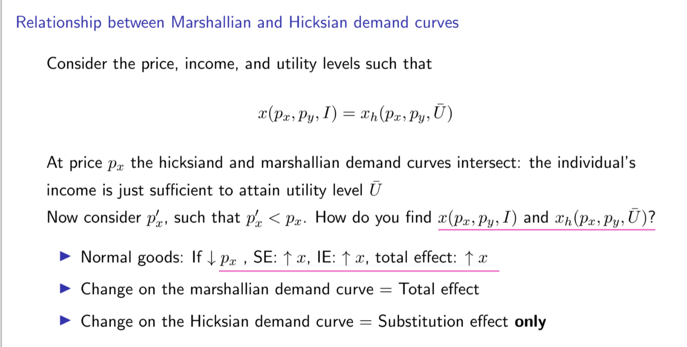
Marshallian to Hicksian and reverse

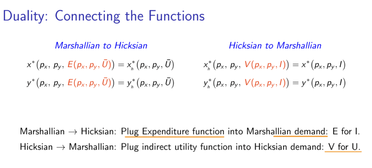
Marshallian demand → Hicksian demand

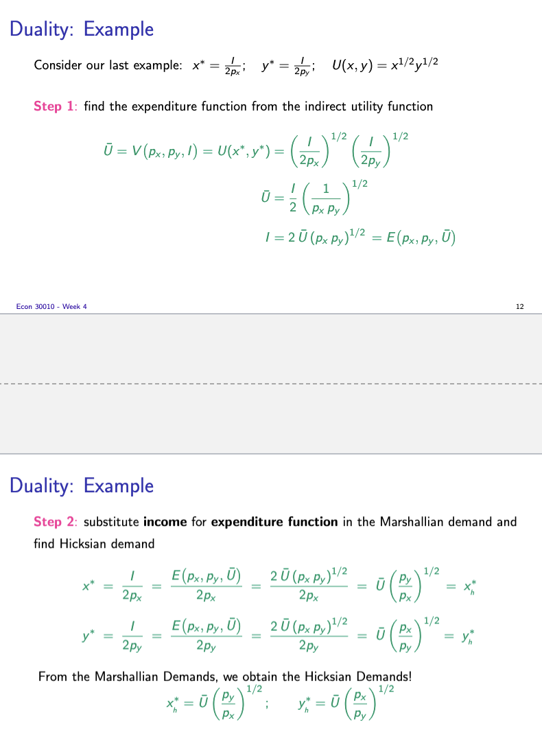
Hicksian Demand → Marshalian Demand

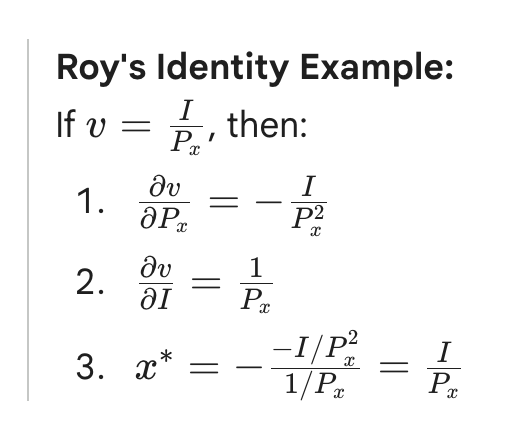
Roy’s Identity

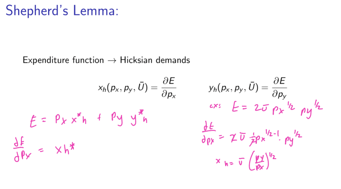
Shepherd’s Lemma

Lump Sum Tax(T)

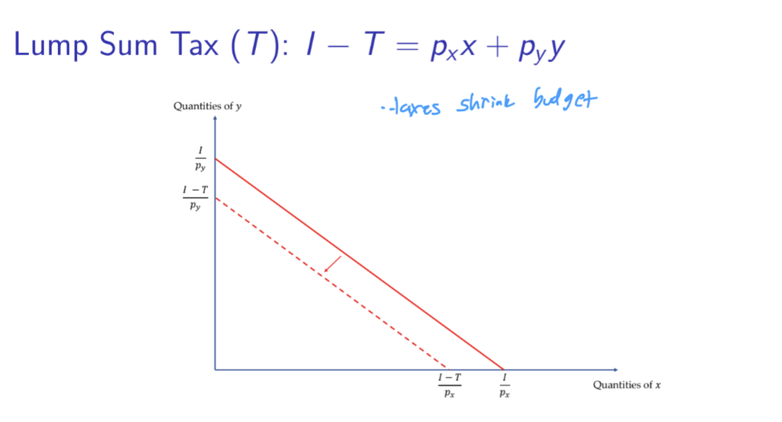
The individual is taxed a fixed amount T regardless of their consumption of goods x and y. I-T= px*x+py*y

Per Unit Tax(t)

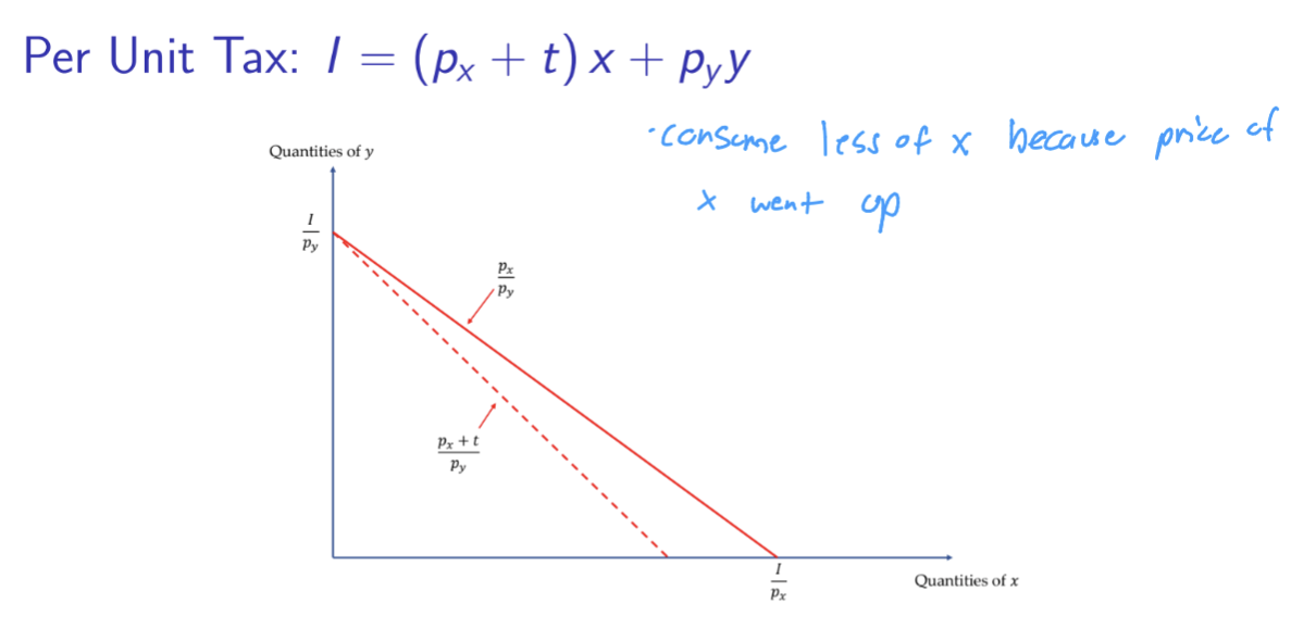
Each unit of good x is taxed a fixed amount t. For example, in Indiana, each 20-pack of cigs is taxed at 0.995. New budget constraint: I = (px+t)*x+py*y

Ad Valorem Tax

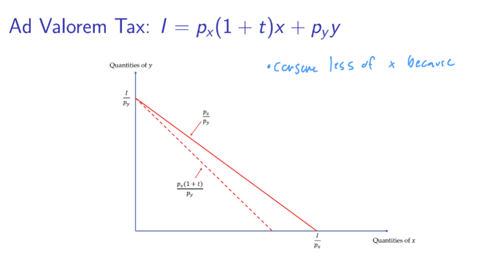
Each unit of good x is taxed at rate t per dollar. For example. if the soda tax rate is 10%, for every dollar spent on soda, the consumer would pay 0.1. New budget constraint: I = px(1+t)*x+py*y

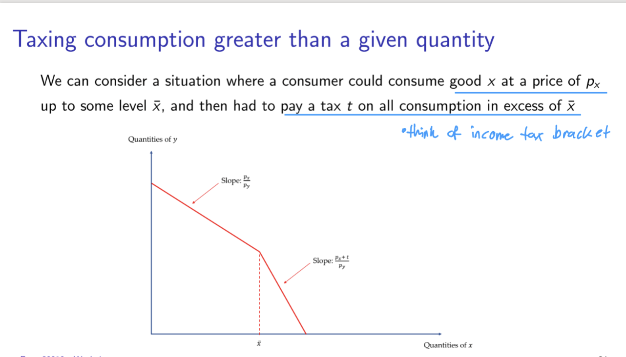
Taxing consumption greater than a given quantity

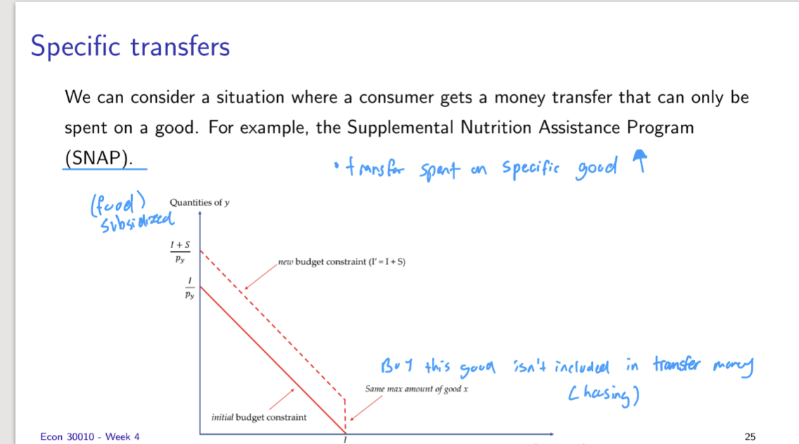
Specific Transfers Graph

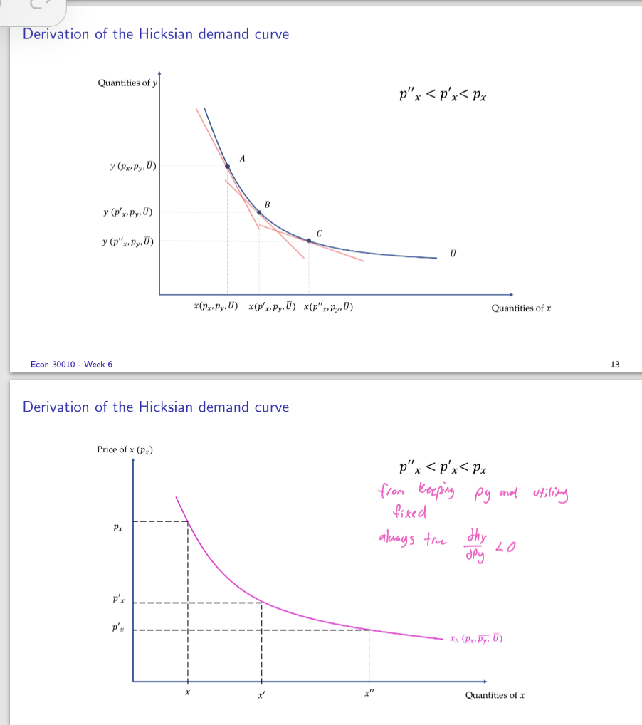
Construction of an Individual’s Demand Curve

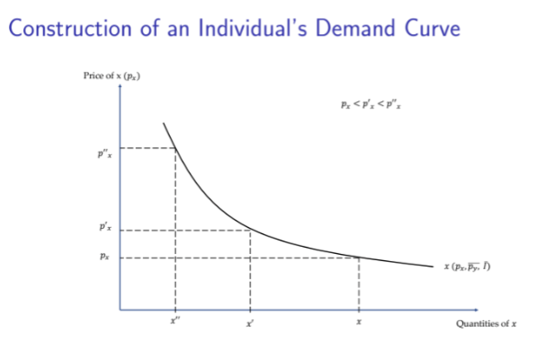
Construction of an Individual's Demand Curve

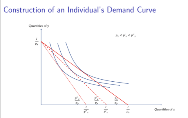
An individual demand curve shows the relationship between the price of a good and the quantity of that good purchased by an individual, holding all other determinants of demand constant [1].

How It's Constructed

The curve is built by examining how quantity demanded changes as the price of a good varies:

• As price increases (from px to p'x to p''x), the quantity demanded decreases (from x to x' to x'') [2]

• This inverse relationship between price and quantity demanded is plotted on a graph with price on the vertical axis and quantity on the horizontal axis [2]

In microeconomic analysis, px might be less than px' if there has been a price increase for good x. When the price of x rises (px' > px), this typically means:

• The budget constraint shifts inward, reducing purchasing power

• Consumers will consume less of x due to the higher price

• The marginal utility per dollar spent on x decreases

This relationship is fundamental to understanding consumer behavior and demand curves in economics.

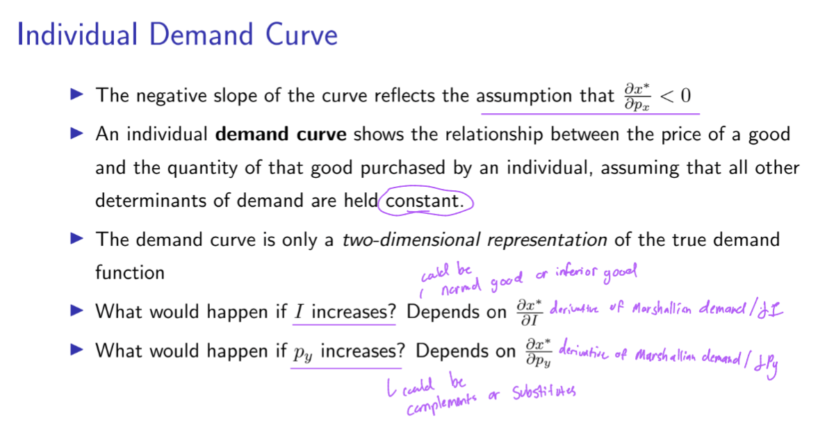
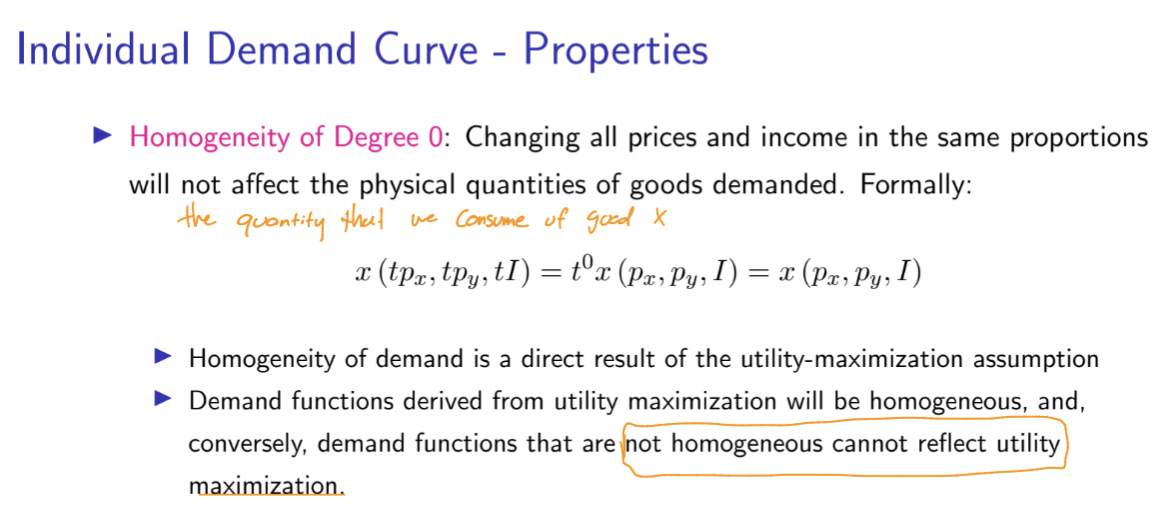
Individual Demand Curve Properties

Changes in Income

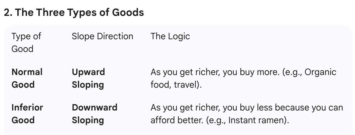
• As a person’s purchasing power increases, it is natural to expect that the quantity of each good purchased will also increase

• Alternate levels of income: I:I < I’ < I’’

• The budget constraint shifts in a parallel way because its slope does not change

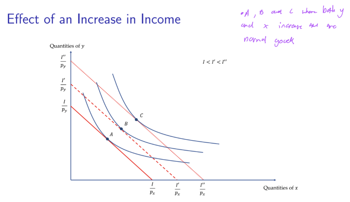
In this case both x and y increase as income increases

dx/dI > 0 and dy/dI > 0

• goods that have this property are called normal goods over some range of income

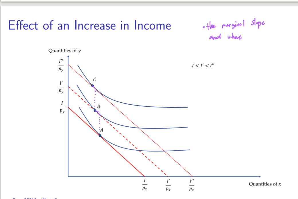
For some goods, however, the quantity chosen may decrease as income increases in some ranges.

• indifference cures do not have to be “oddly” shaped to exhibit inferiority

• the curves can continue to obey the assumption of diminishing MRS

• example: potatoes, ramen

• Goods that have this property are called inferior goods over some range of income

• dx/dI < 0 or dy/dI < 0

• In this model both goods can’t be inferior - only one

  

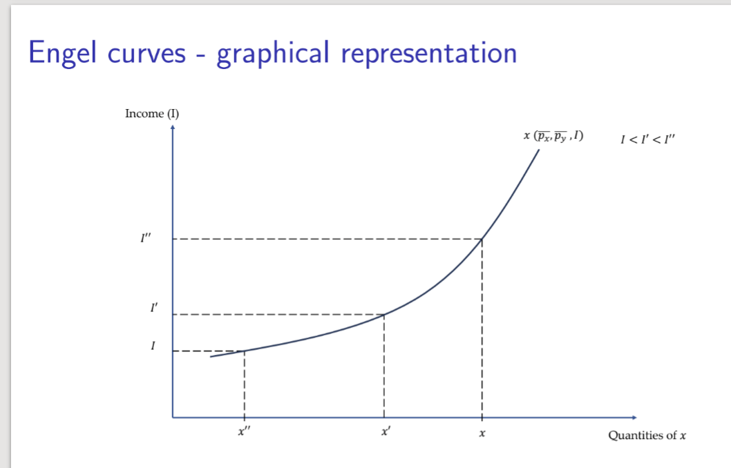
Engel curves

• describe how household expenditure on particular goods or services depends on household income

• is a graph of the optimal good x a function of income I, with all prices behing held constant (px, py)

inferior would look like:

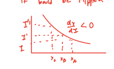
1. How to Read the Graph

• Axes: Usually, Income (I) is on the horizontal (x-axis) and the Quantity of the good (q) is on the vertical (y-axis).

• The Slope: The direction of the slope tells you exactly what kind of good you are dealing with.

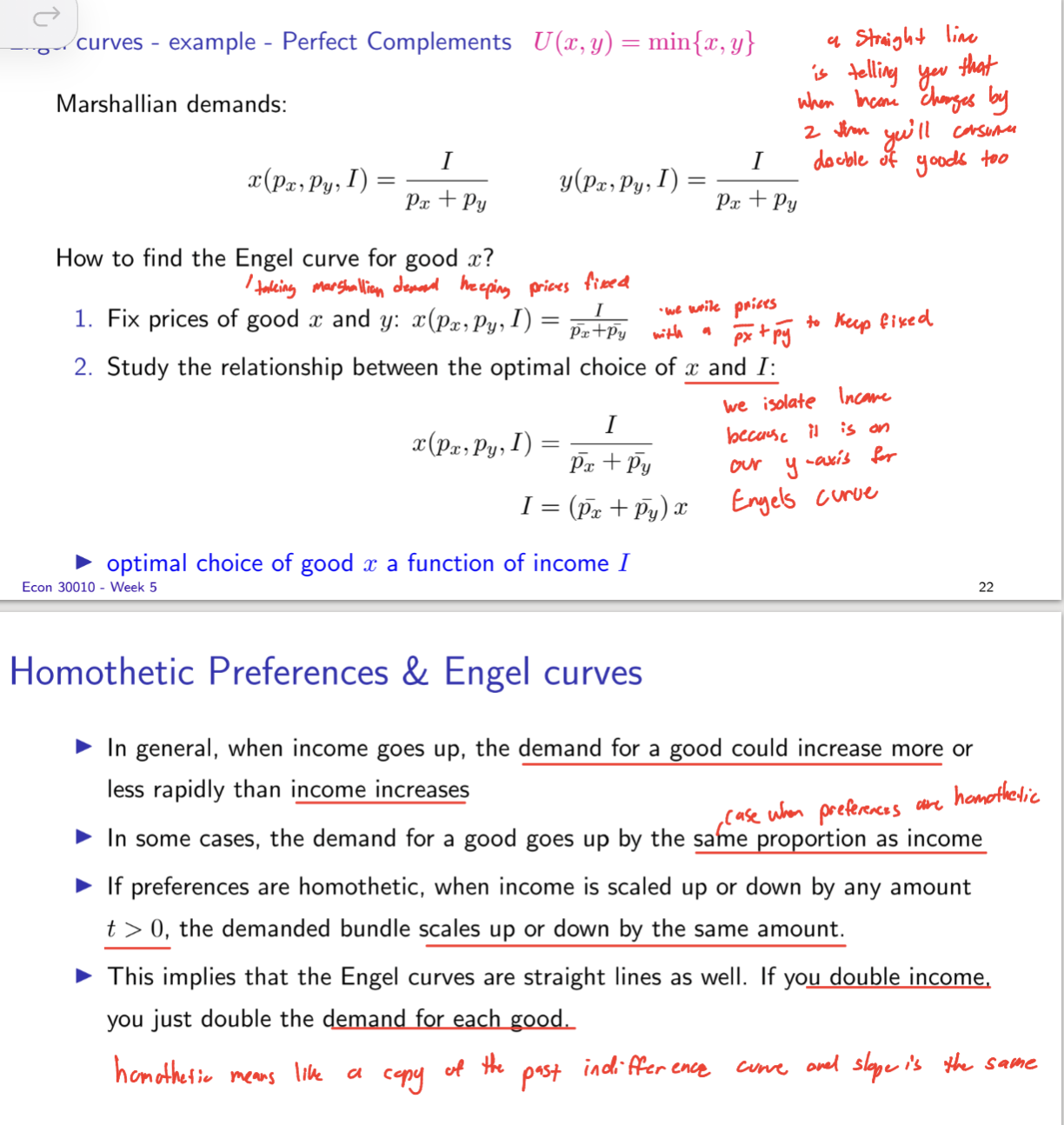
Engel Curves - Perfect Complements

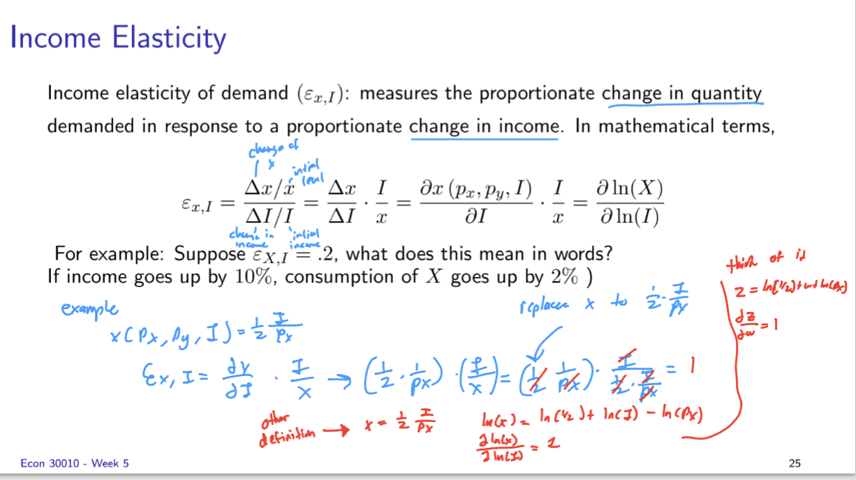
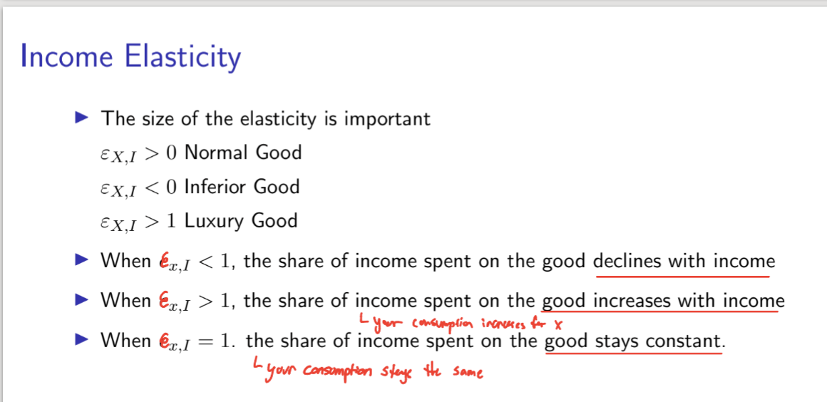
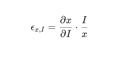
Income Elasticity

Elasticities: state how much one thing changes with respect to another.

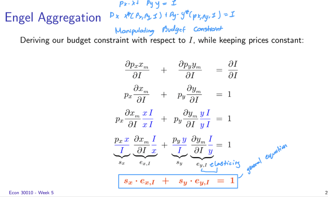
Engel Aggregation

• sx and sy: The share of your budget spent on each good (e.g., 0.6 for 60%).

• exI and eyI: The income elasticity of each good.

3. Why it matters (The "Intuition")

This formula tells us that you cannot have only inferior goods.

• If you get richer and buy less of Good x (inferior), you must be buying more of Good y to make up for it and spend your new income.

• Mathematically, if one elasticity is negative, the other one has to be large enough and positive to make the whole equation equal 1.

Engel Aggregation:

• Definition: The budget-weighted sum of income elasticities equals 1.

• Formula:

  

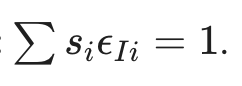
• Key Lesson: If income goes up by 1%, total spending must also go up by 1%. You can't be "inferior" in everything you buy.

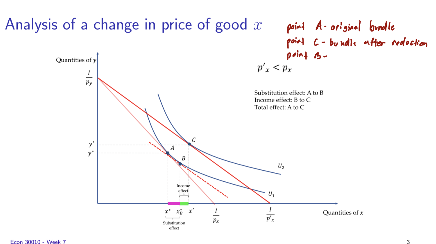
Price Changes

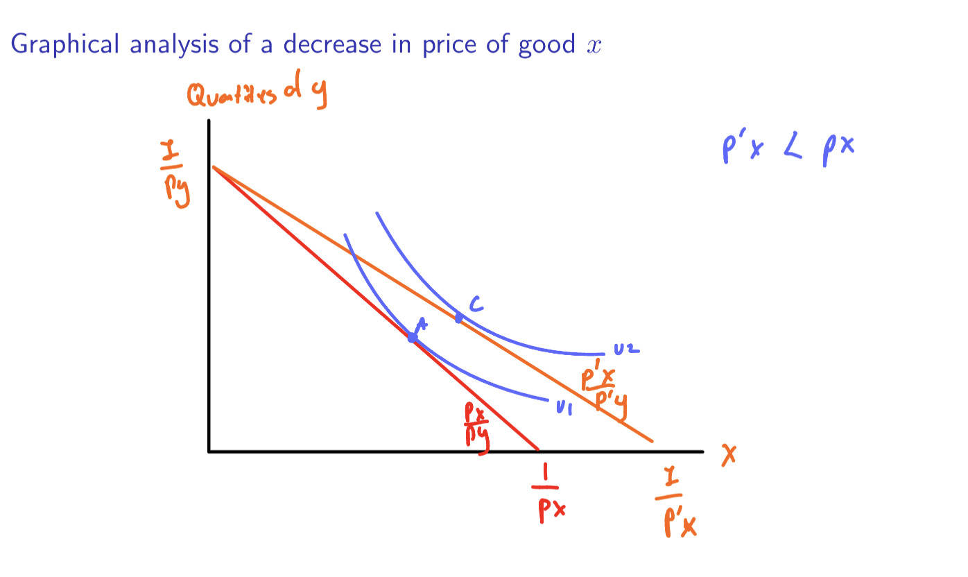
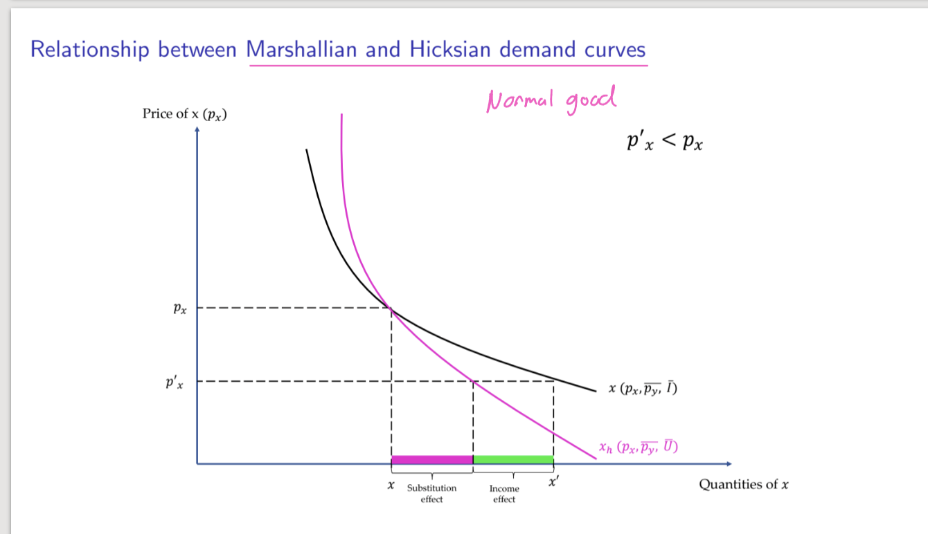
Income and Substitution effects on a Normal Good

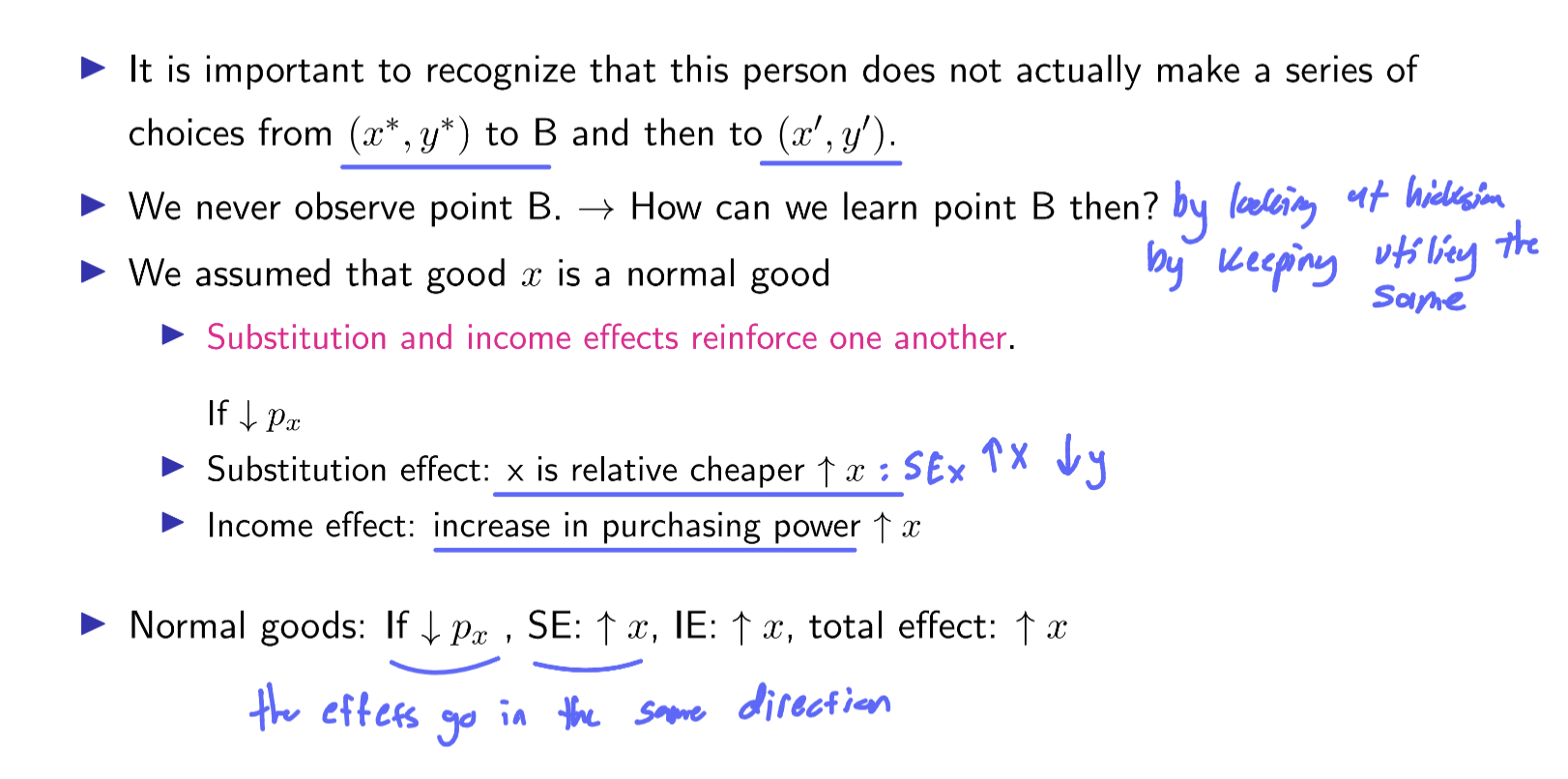
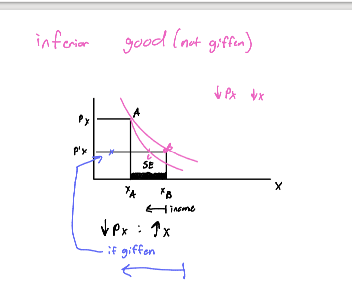
Income and Substitution on Inferior Good

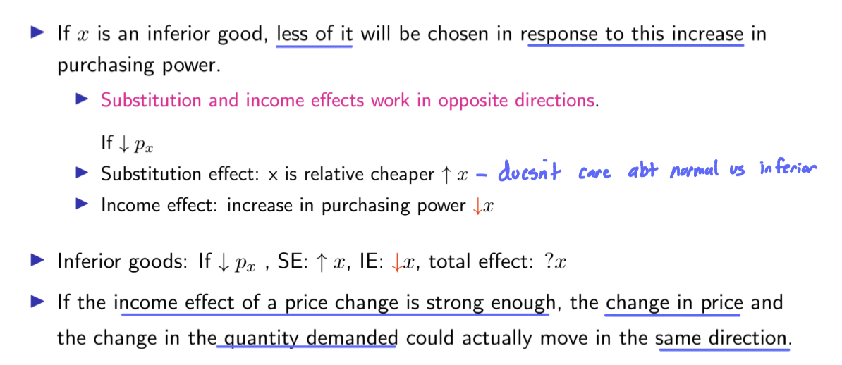
For most inferior goods, the Substitution Effect is still stronger than the Income Effect. So, even though the "Income Effect" arrow points down, the total consumption usually still goes up—just not as much as it would for a normal good.

Giffen Good’s

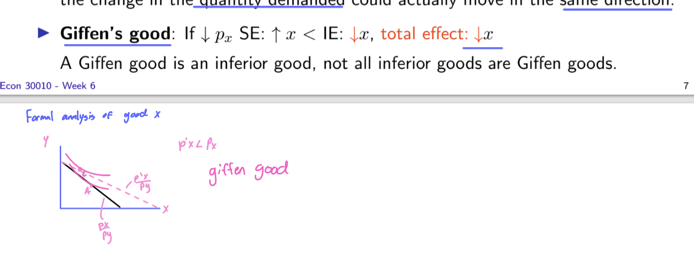
A Giffen Good is an extremely inferior good where the negative Income Effect is so powerful that it completely overwhelms the Substitution Effect.

• When the price goes down, you actually buy less of it. When the price goes up, you buy more.

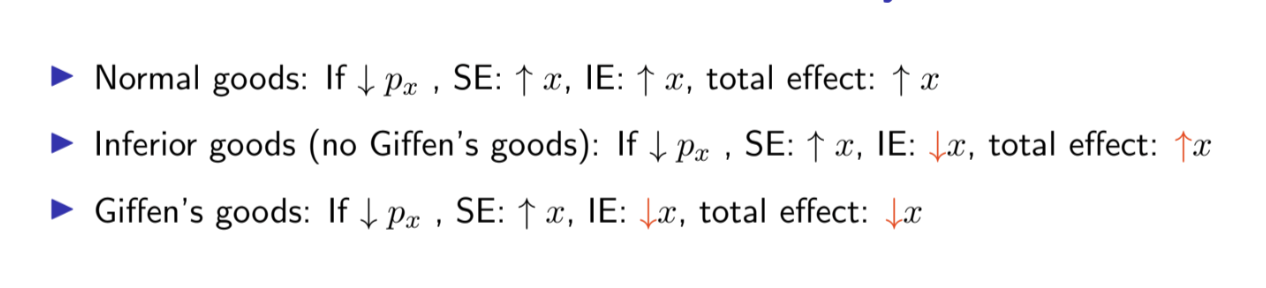
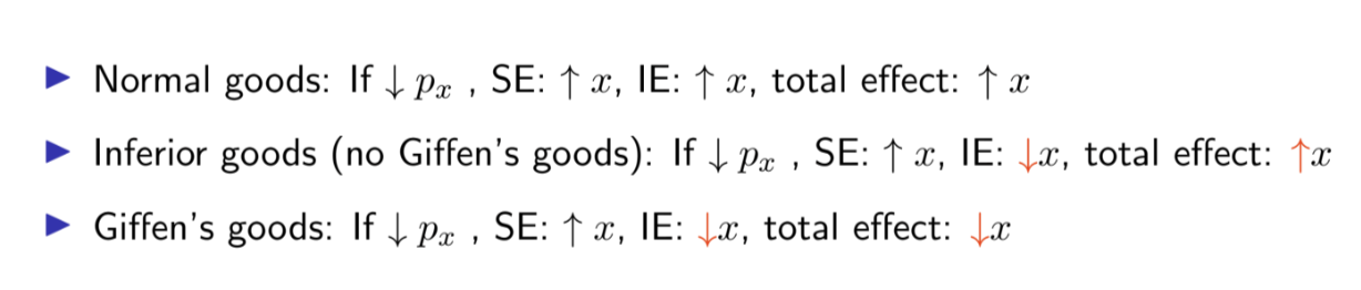
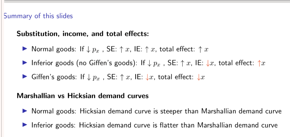
Total effects | Substitution effect | Income effect

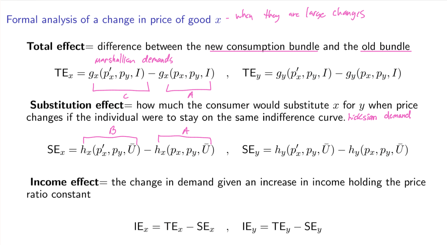
Slutsky Equation

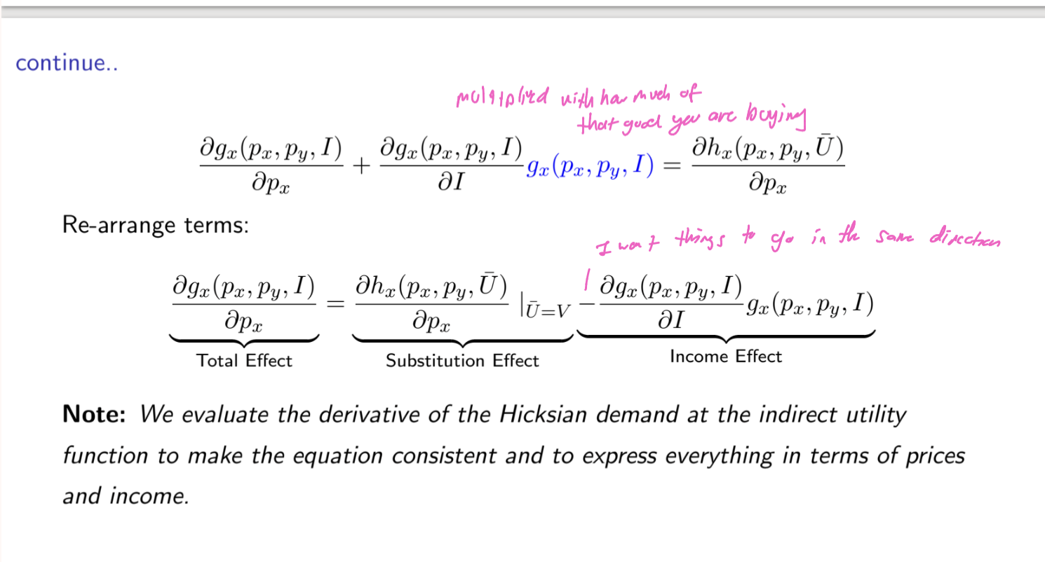
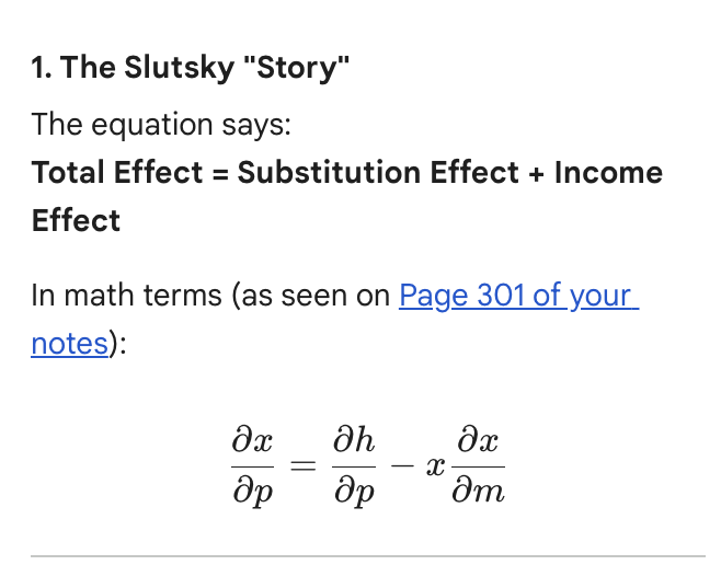
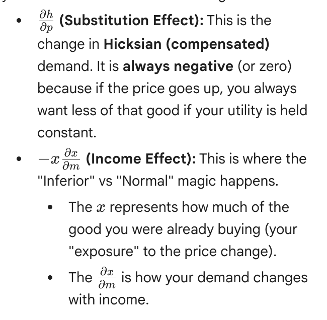
Good Type	Sub Effect	Income Effect	Total Effect
Normal	Negative (-)	Negative (-)	Always Negative (-) (Law of Demand holds)
Inferior	Negative (-)	Positive (+)	Usually Negative (-) (SE > IE)
Giffen	Negative (-)	Positive (+)	Positive (+) (IE > SE, Law of Demand fails)

Hicksian Demand Curve

The "Compensated" Logic

Think of it this way:

1. Price Drops: You are now "richer" because your money goes further.

2. The Thought Experiment: To isolate the Substitution Effect, the professor "compensates" for that price drop by taking away just enough of your income so that you are no better off than you were before (keeping you on the same Indifference Curve).

3. The Result: Even though you have less money now (because it was taken away), you still buy more of Good X because it is relatively cheaper than Good Y

Relationship between Marshallian and Hicksian demand curves

Summary of Substitution, income, and total effects

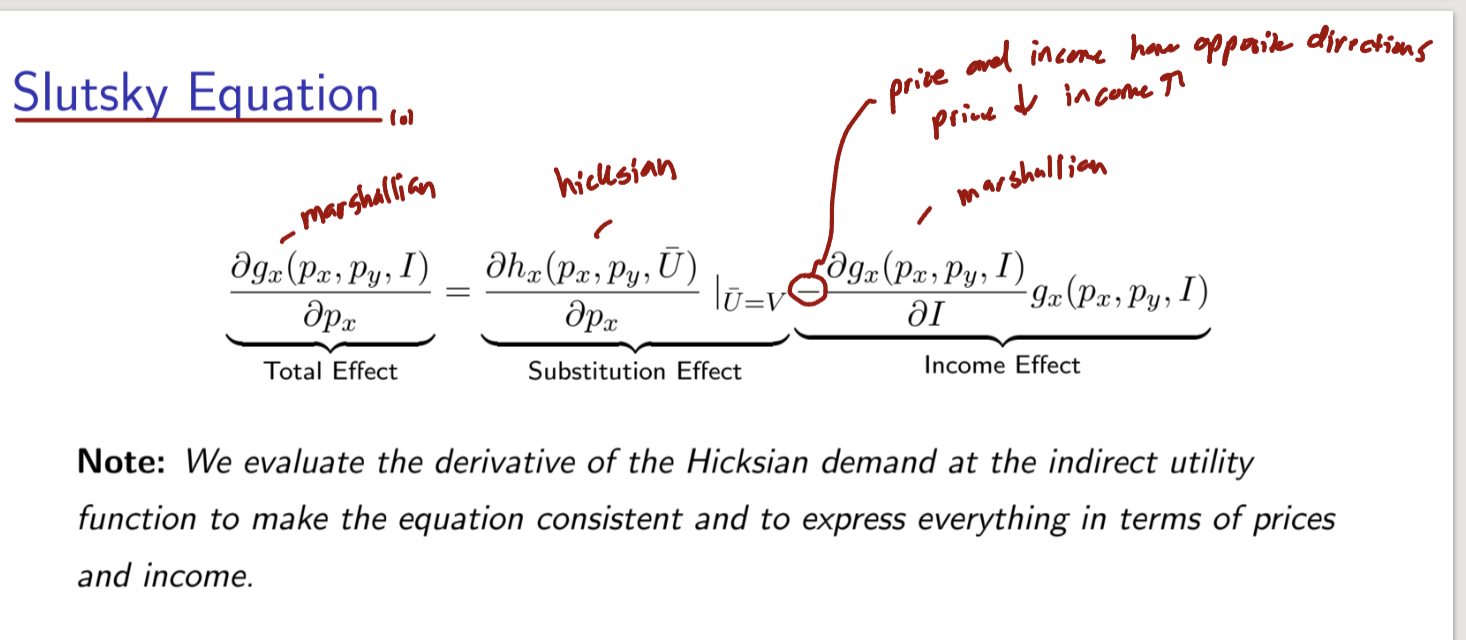
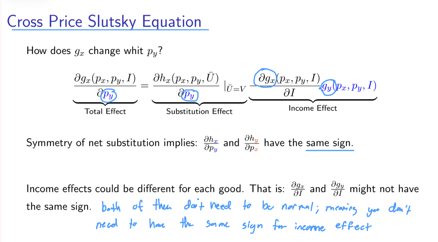
Cross Price Slutsky Equation

3. Decoding the "Symmetry" Note

Your slide mentions that "Symmetry of net substitution implies $\frac{\partial h_x}{\partial p_y}$ and $\frac{\partial h_y}{\partial p_x}$ have the same sign."

• This is a "math gift" for your exam. It means if Apple is a substitute for Orange in the Hicksian world, then Orange must be a substitute for Apple. They can't "disagree."

• However, the Total Effect (Marshallian) doesn't have to be symmetric! One could be a substitute and the other a complement because their Income Effects might be totally different sizes1. The Question being asked

Instead of "If the price of apples falls, do I buy more apples?", this slide asks: "If the price of oranges ($p_y$) changes, what happens to my demand for apples ($g_x$)?"

2. The Two Forces at Play

• The Substitution Effect (Cross-Price): If oranges get expensive, you swap them for apples. This is the $\frac{\partial h_x}{\partial p_y}$ part.

  • Net Substitutes: If this value is positive, the goods are substitutes (Price of $Y \uparrow \rightarrow$ Demand for $X \uparrow$).

  • Net Complements: If this value is negative, they are complements (Price of $Y \uparrow \rightarrow$ Demand for $X \downarrow$).

• The Income Effect (Cross-Price): This is the part that usually confuses students. If the price of oranges ($p_y$) goes up, you are effectively poorer because you spend a chunk of your budget on oranges ($g_y$).

  • This "loss of wealth" then affects how many apples you buy.

3. Decoding the "Symmetry" Note

Your slide mentions that "Symmetry of net substitution implies $\frac{\partial h_x}{\partial p_y}$ and $\frac{\partial h_y}{\partial p_x}$ have the same sign."

• This is a "math gift" for your exam. It means if Apple is a substitute for Orange in the Hicksian world, then Orange must be a substitute for Apple. They can't "disagree."

• However, the Total Effect (Marshallian) doesn't have to be symmetric! One could be a substitute and the other a complement because their Income Effects might be totally different sizes

Elasticity of Demand

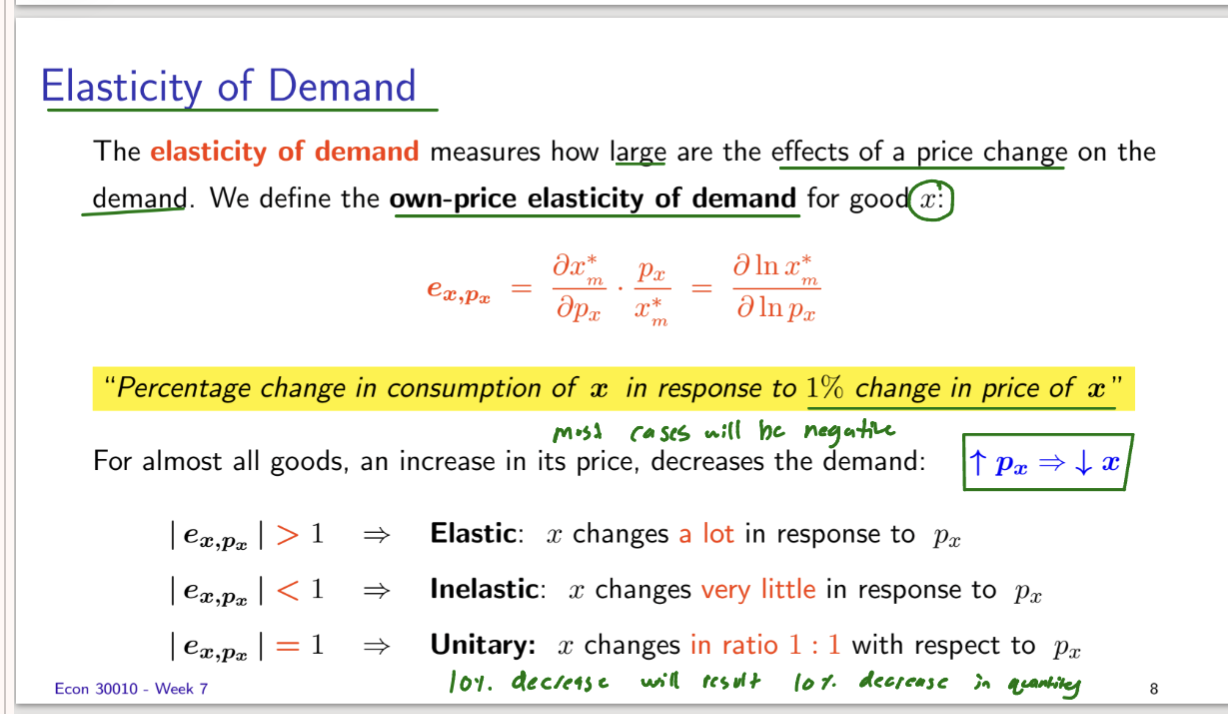
dx*m means marshallian demand

• it includes both the substitution effect and income effect

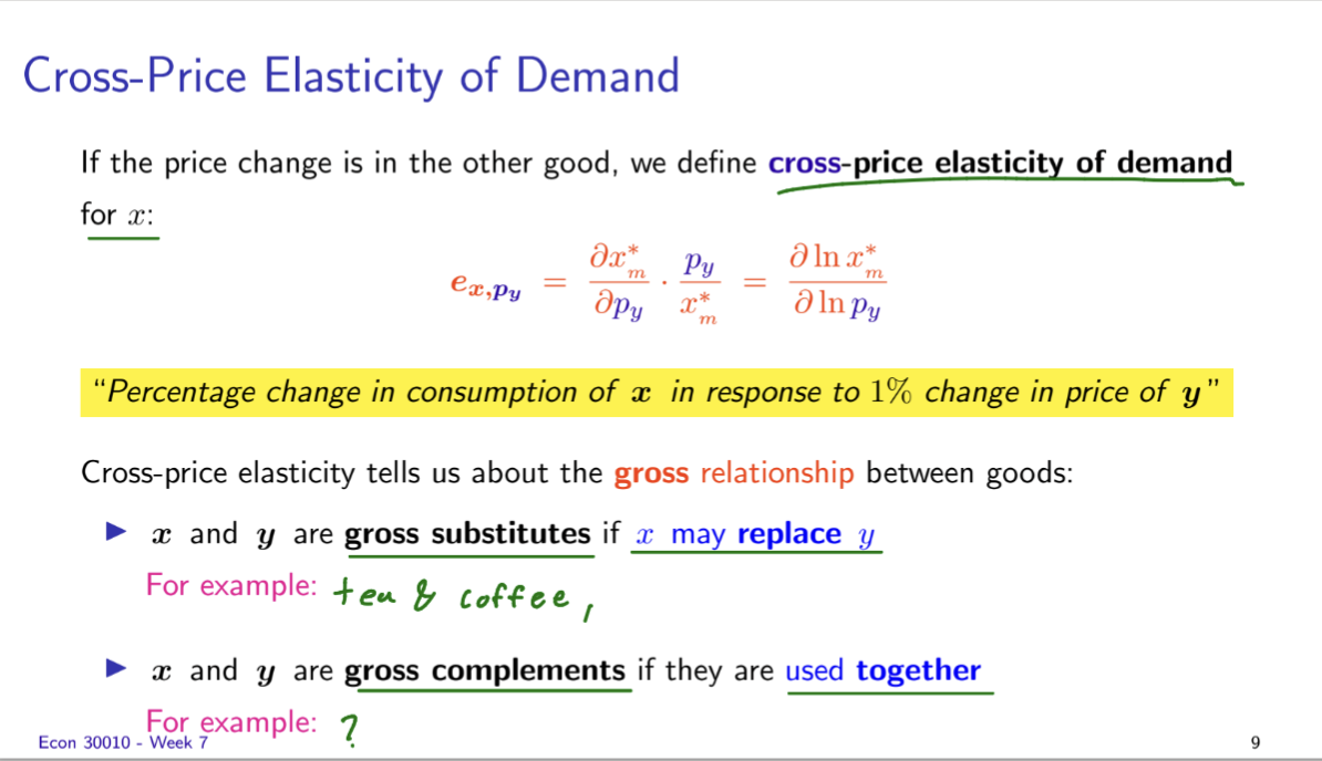
Cross-Price Elasticity of Demand and Gross Substitutes/complements

Gross Substitution

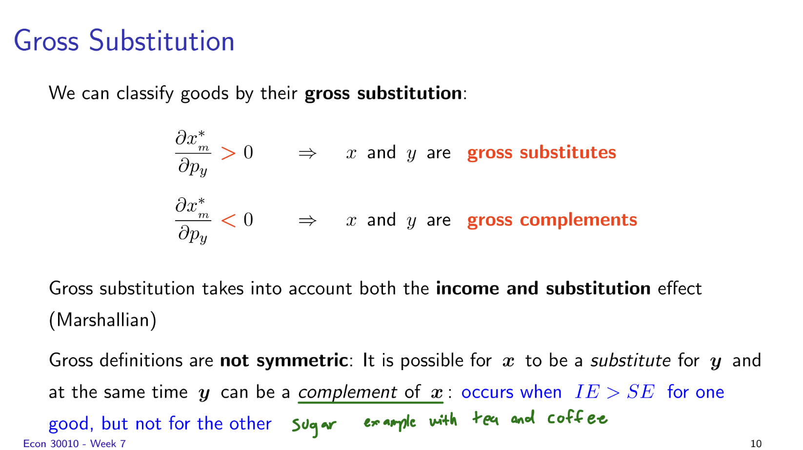
• if our cross price elasticity is above 0 then our x and y are gross substitutes.

• if our cross price elasticity is less than 0 then our x and y are gross complements

Compensated Price Elasticity of Demand

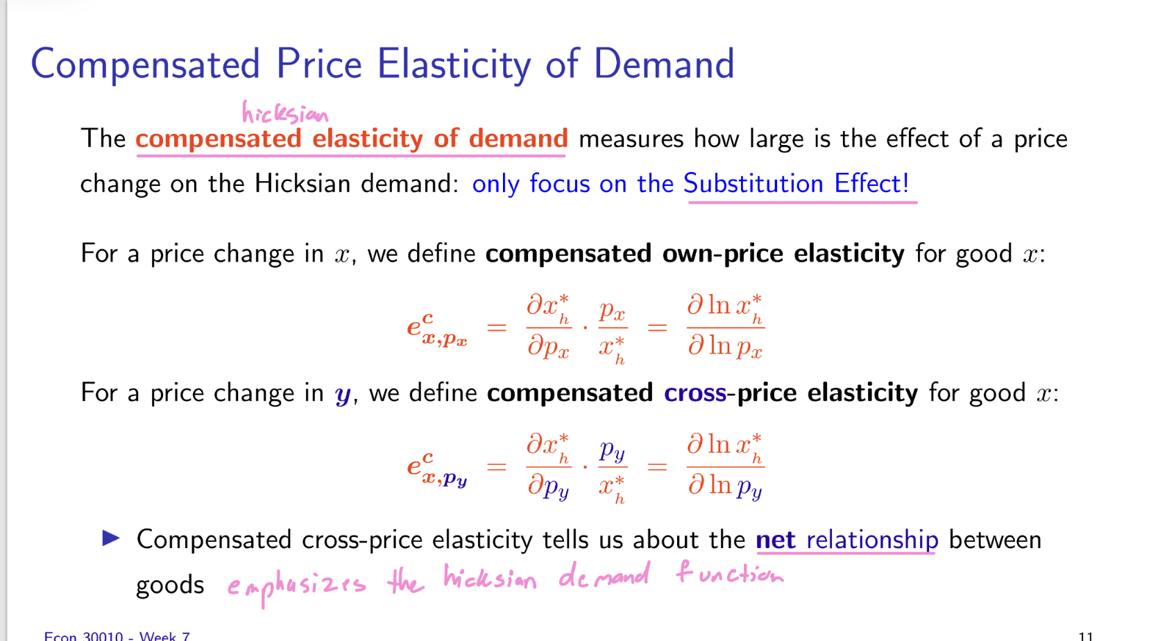
• the dx*h is the hicksian demand

• tells us if they are net substitutes or net complements

Net Substitution

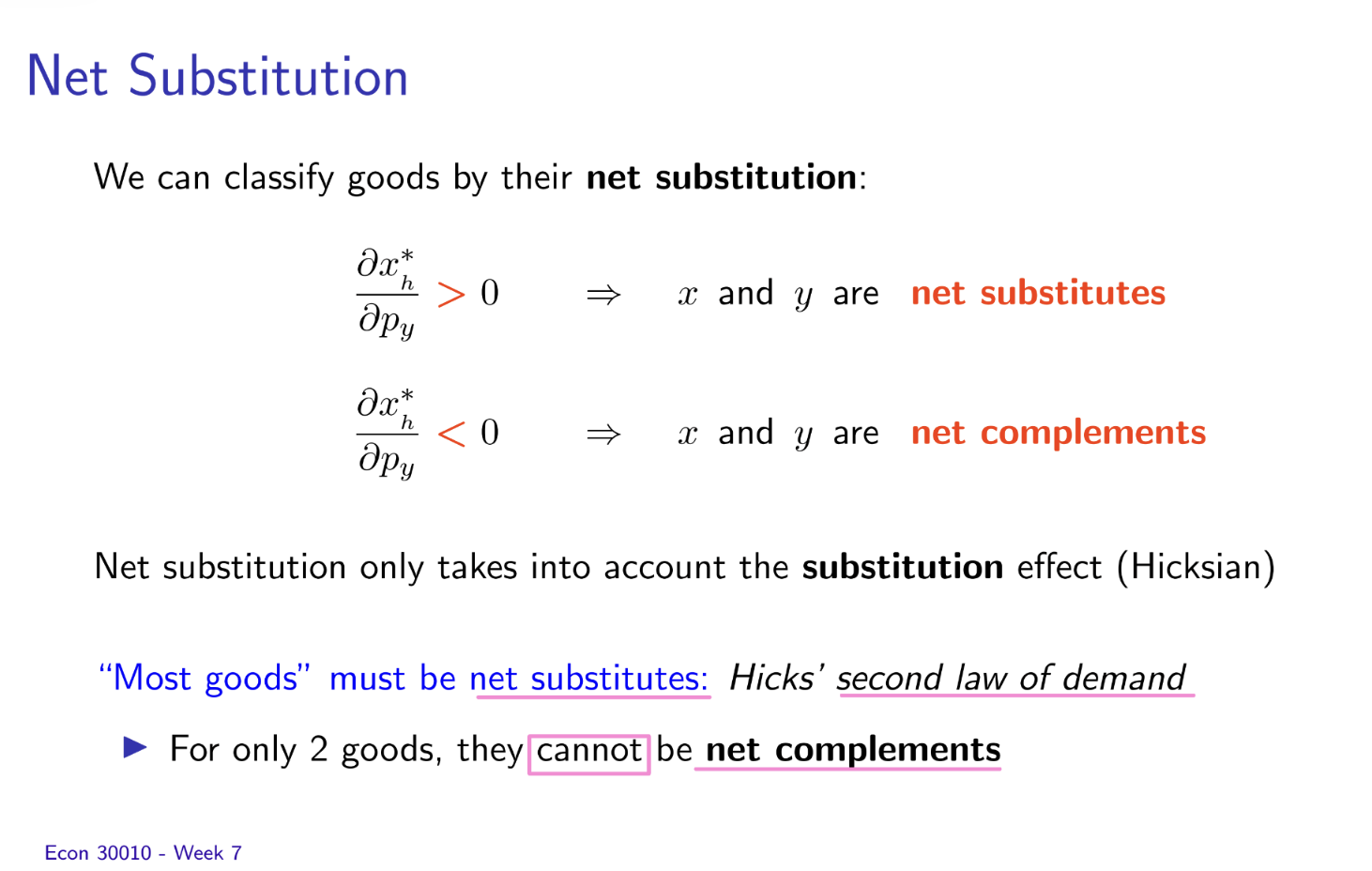
• compensated cross-price elasticity of demand is used to determine net substitution

• if compensated cross-price elasticity of demand is above 0 then x and y are net substitutes

• if compensated cross-price elasticity of demand is below 0 then x and y are net complements

• 2 goods, cannot be net complements because this only pays attention to the substitution effect so if you consume less of y then you have to consume more of x to stay on the same utility curve

• is it always true that (image)?

  

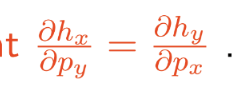
• The Result: The "substitution effect" of a change in Py on the demand for x is identical to the "substitution effect" of a change in Px on the demand for y.

Relationships between Elasticities

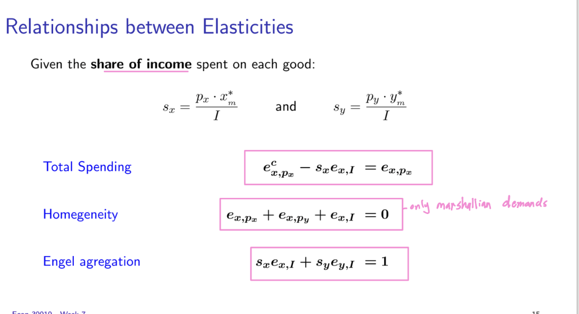
ex, I means income elasticity of demand.

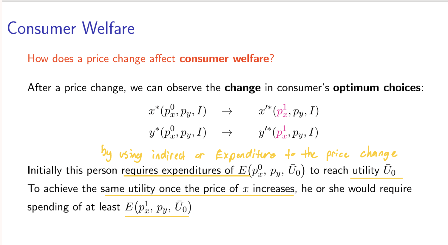
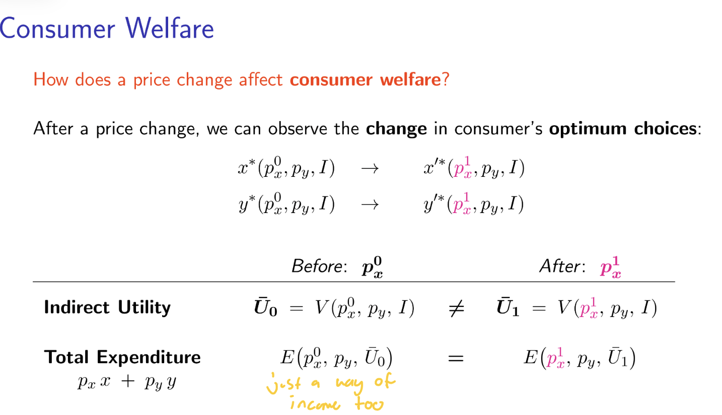
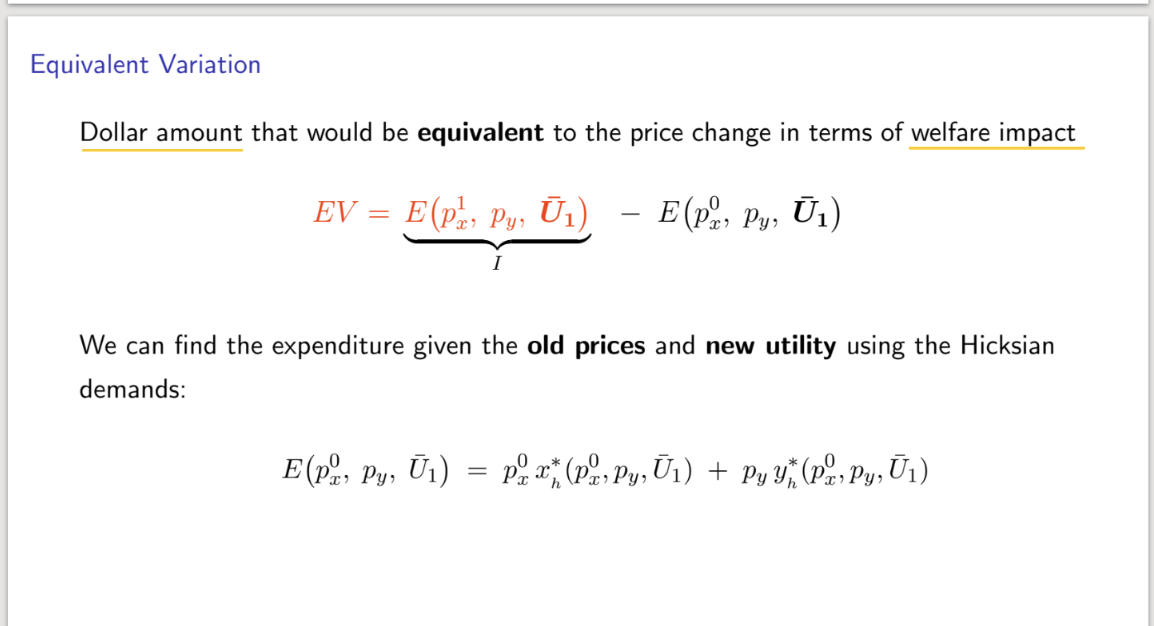
Consumer Welfare

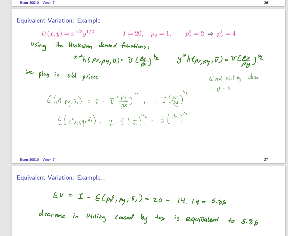
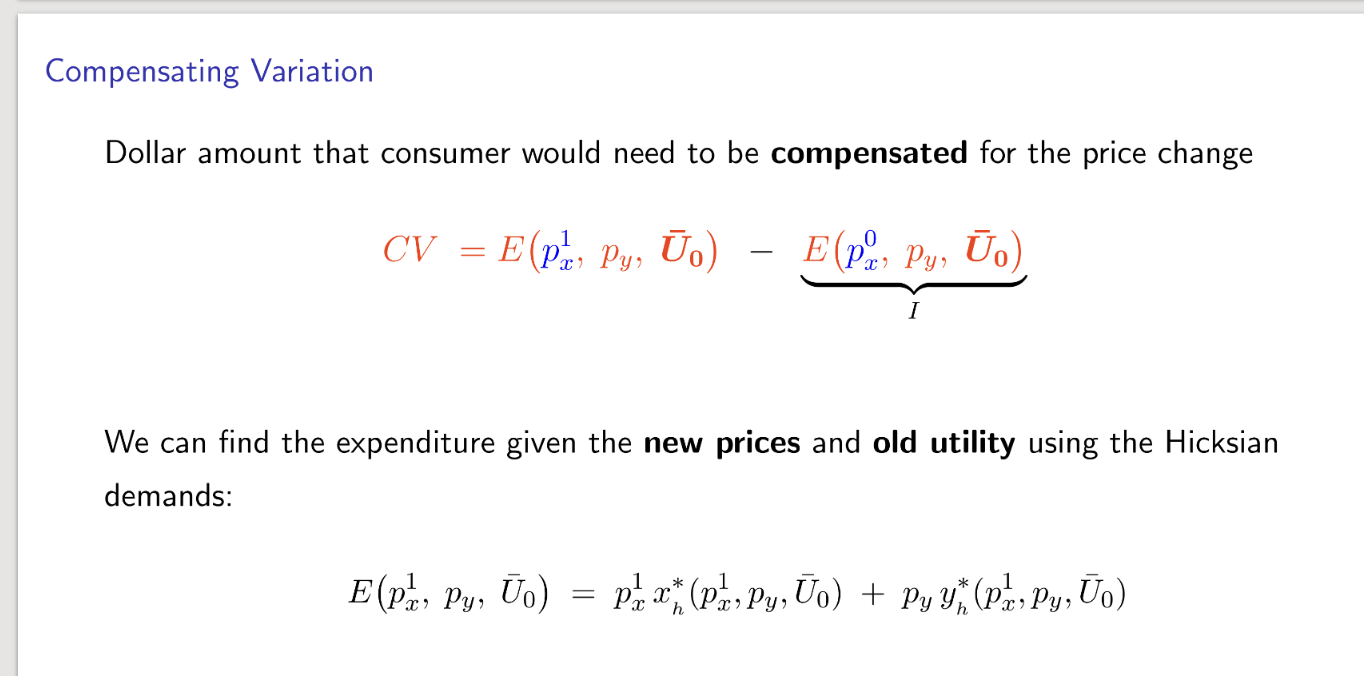
Equivalent Variation

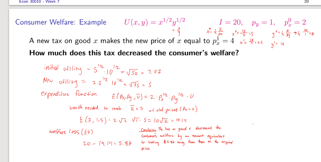
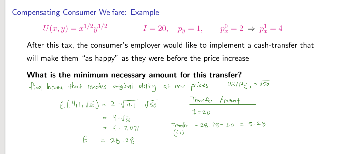
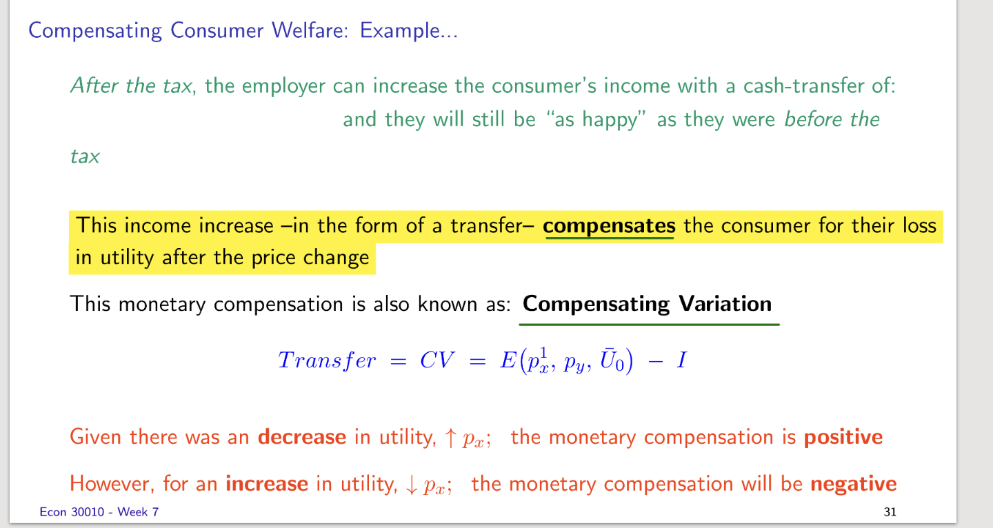
Compensating Consumer Welfare: Example

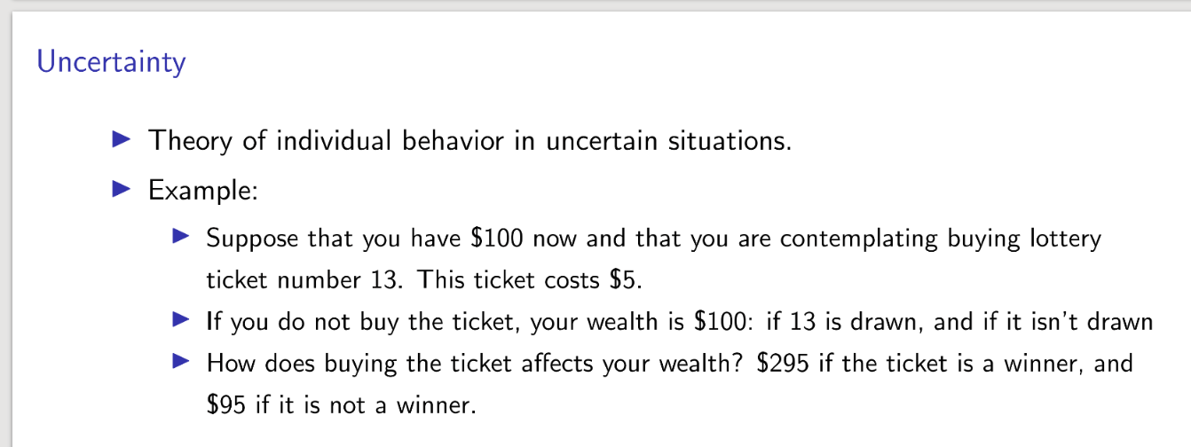
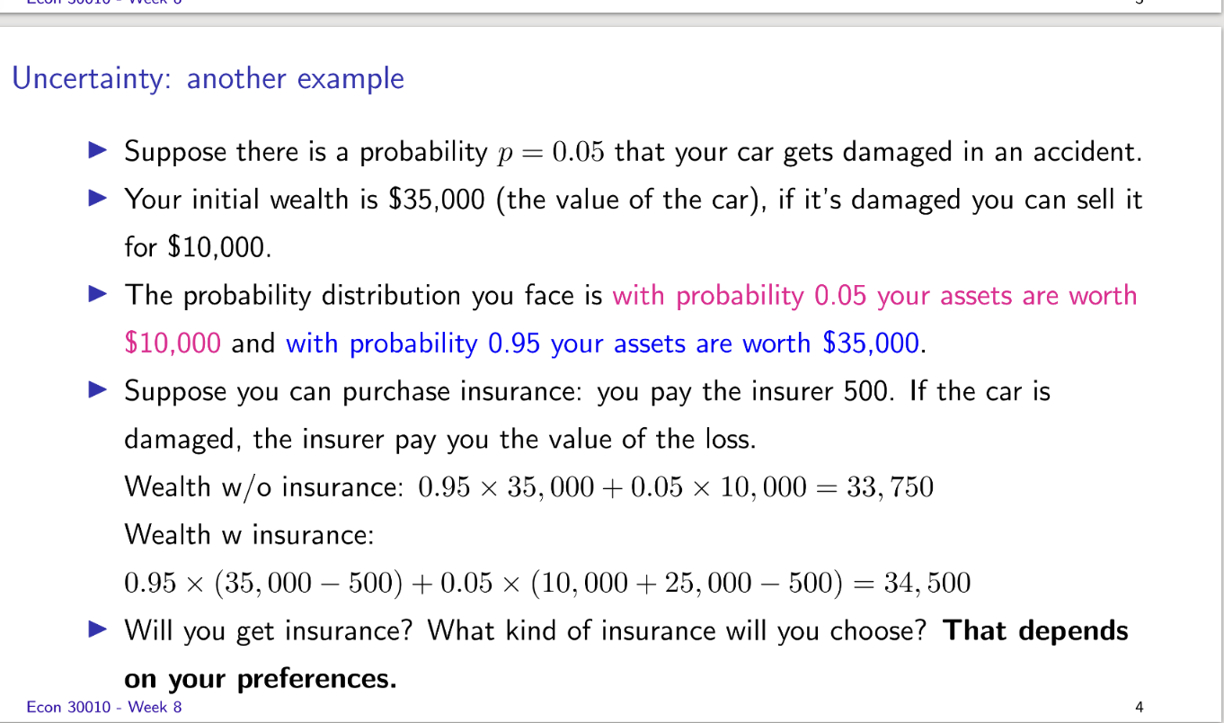
Uncertainty

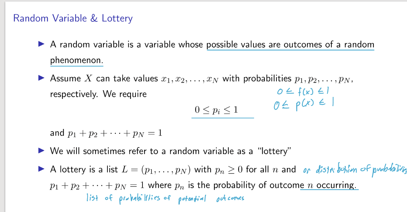
Random Variable and Lottery

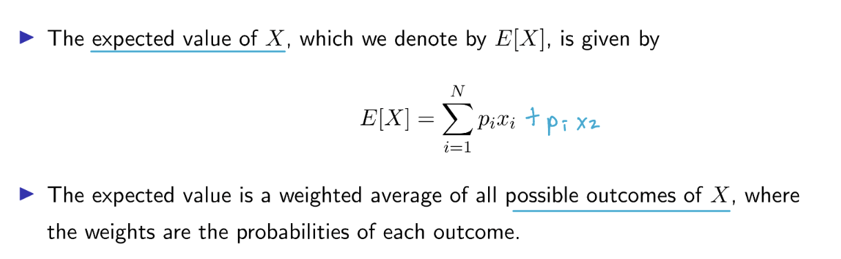
Expected Value

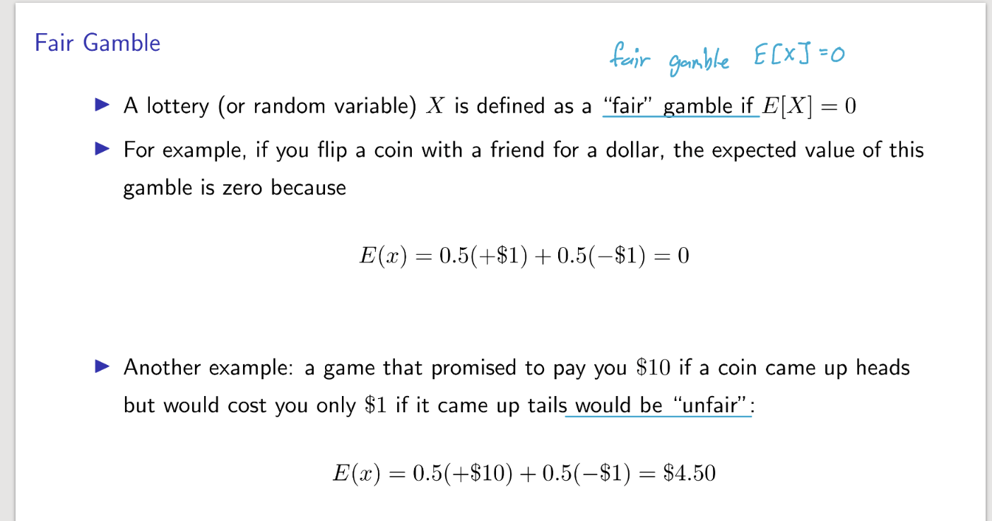
Fair Gamble

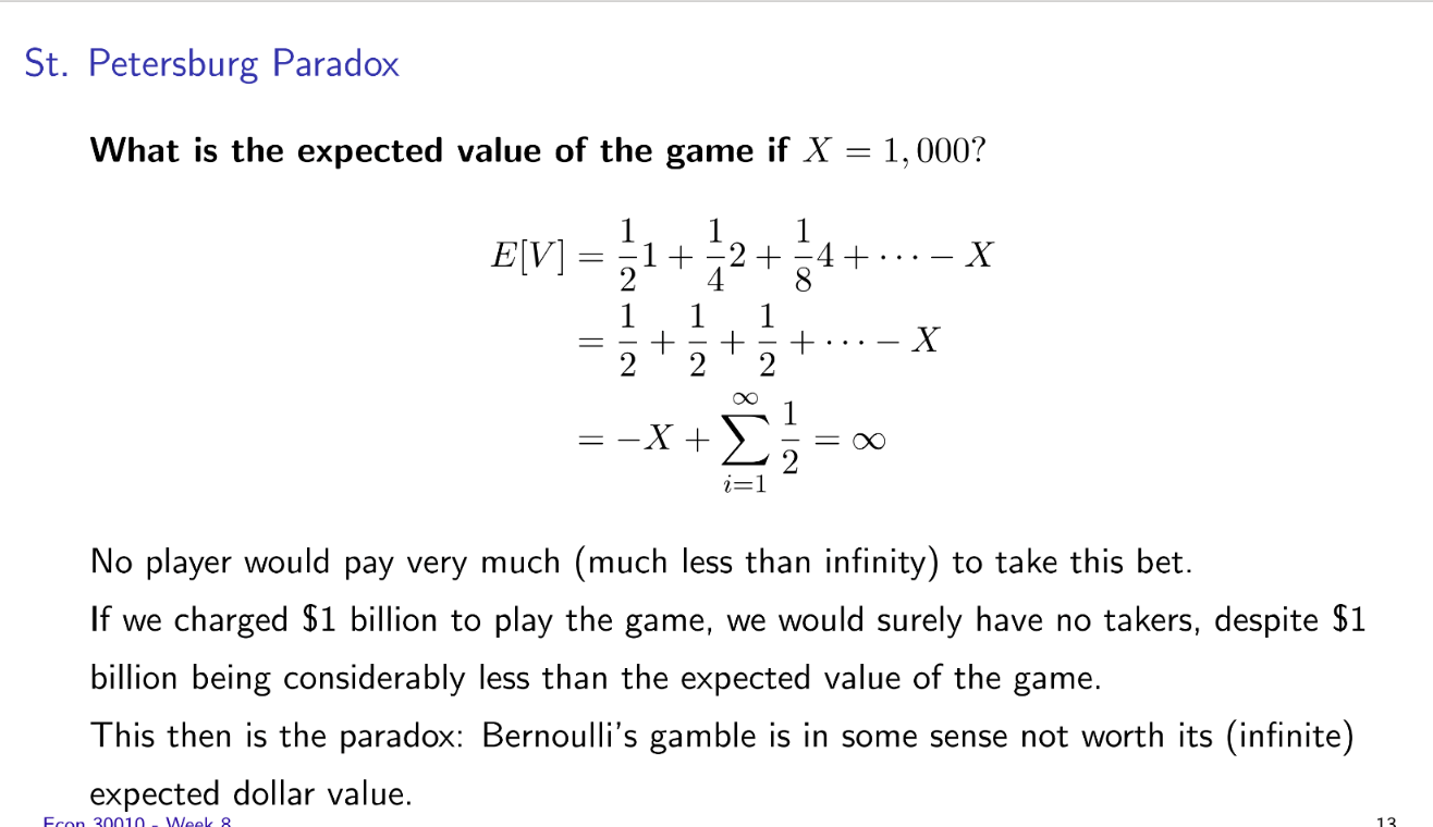
St. Petersburg Paradox

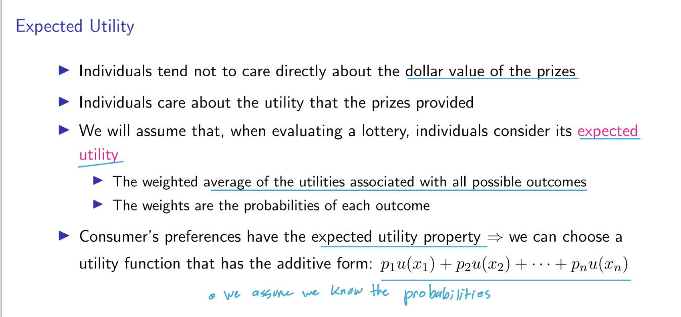
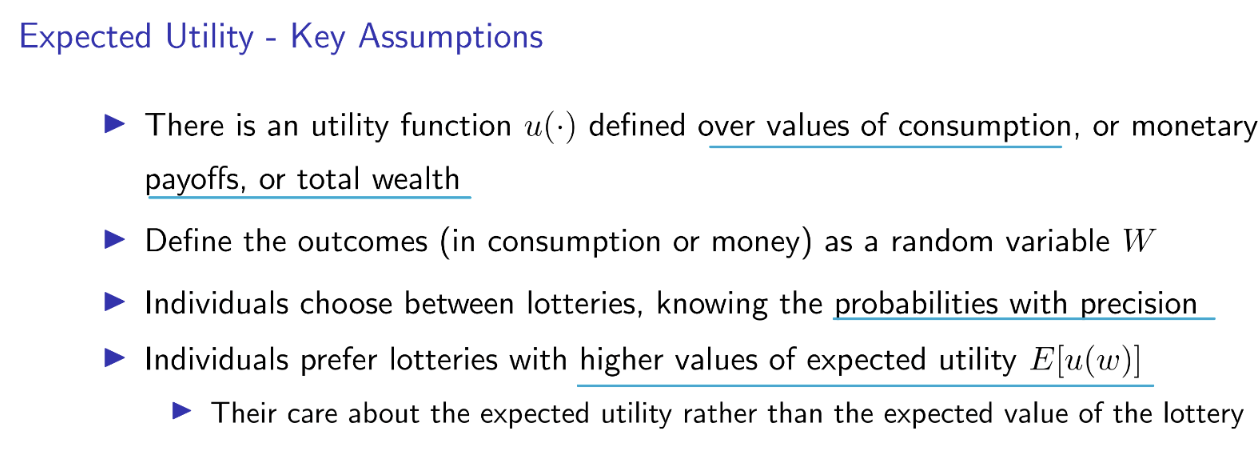
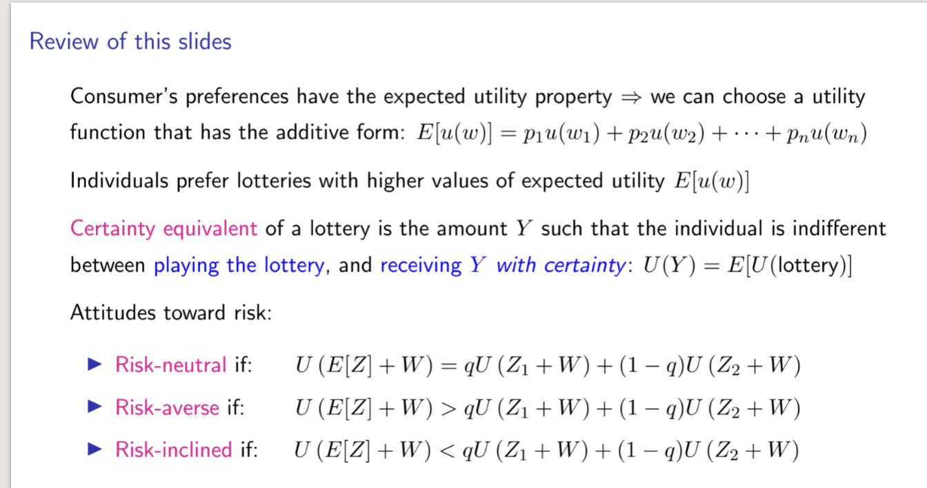
Expected Utility

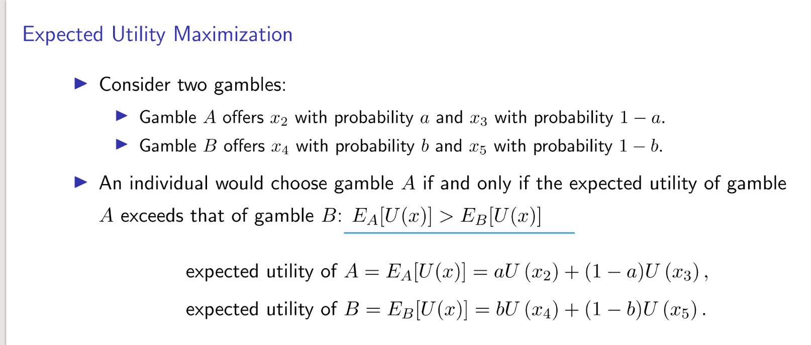
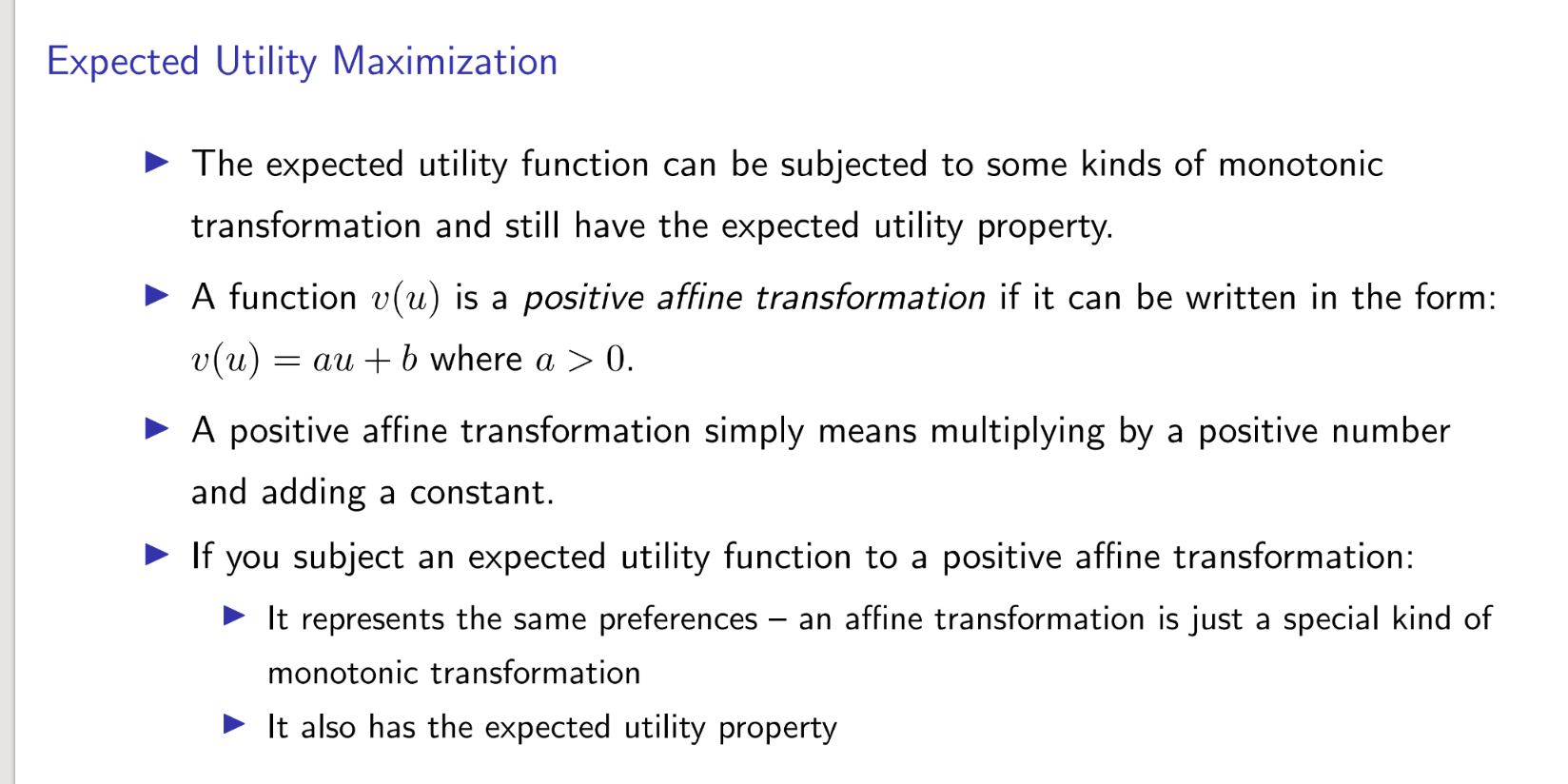
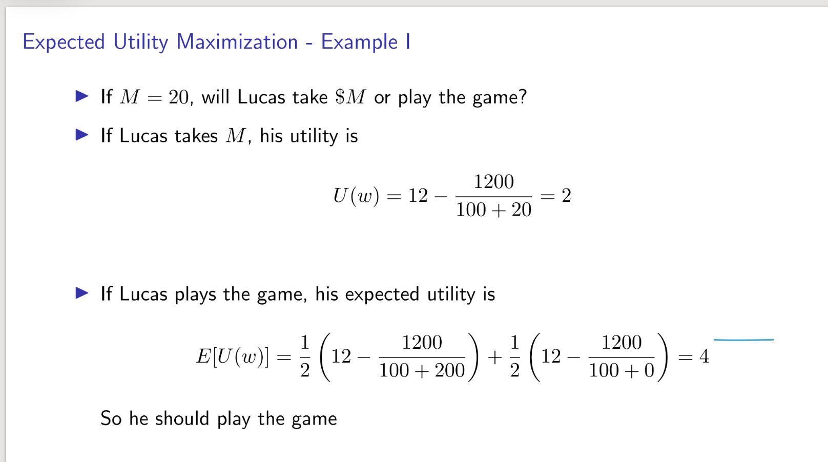
Expected Utility Maximization

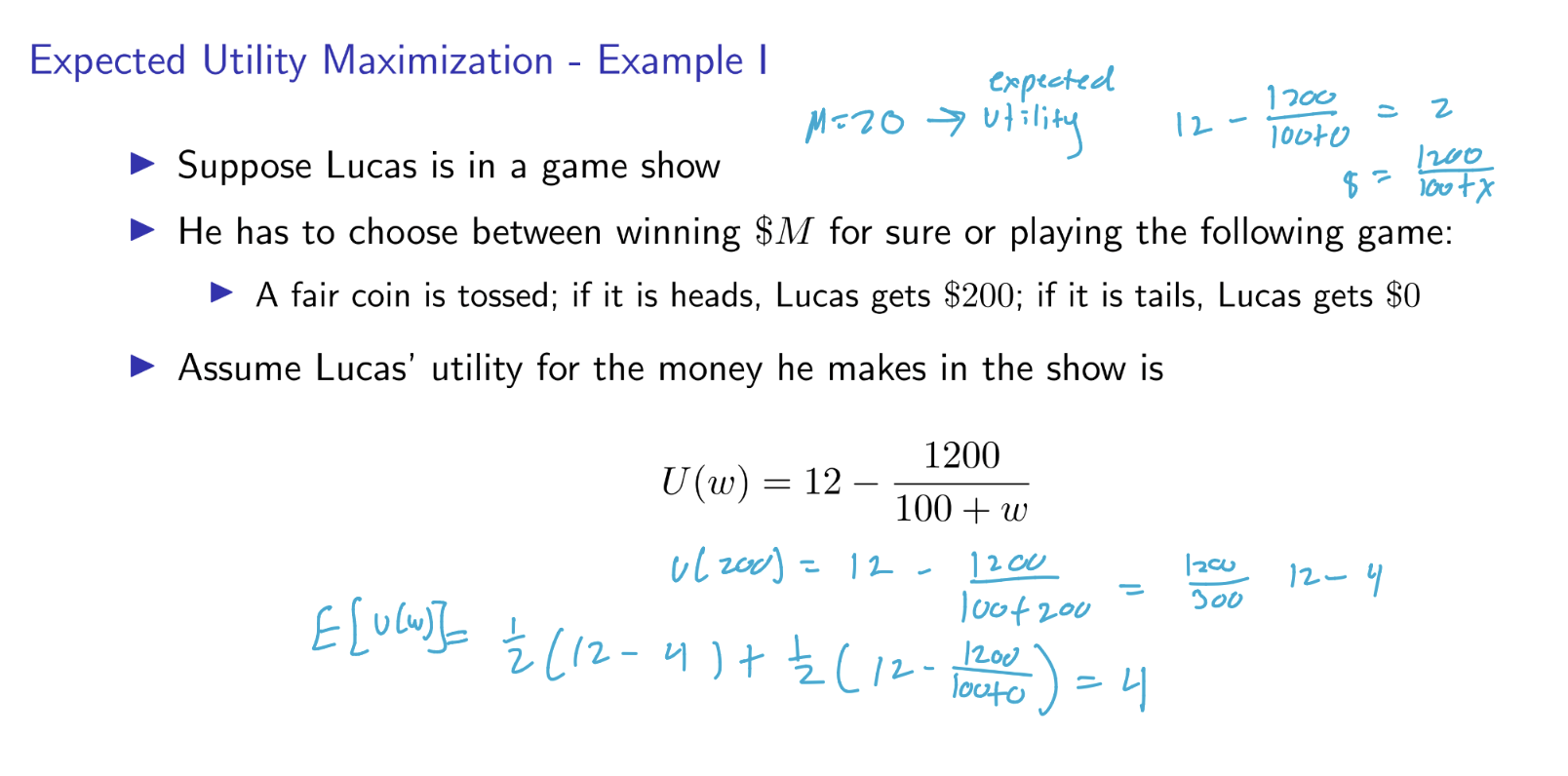
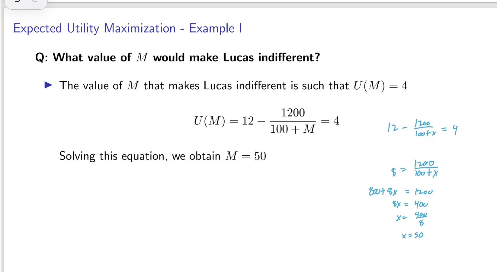
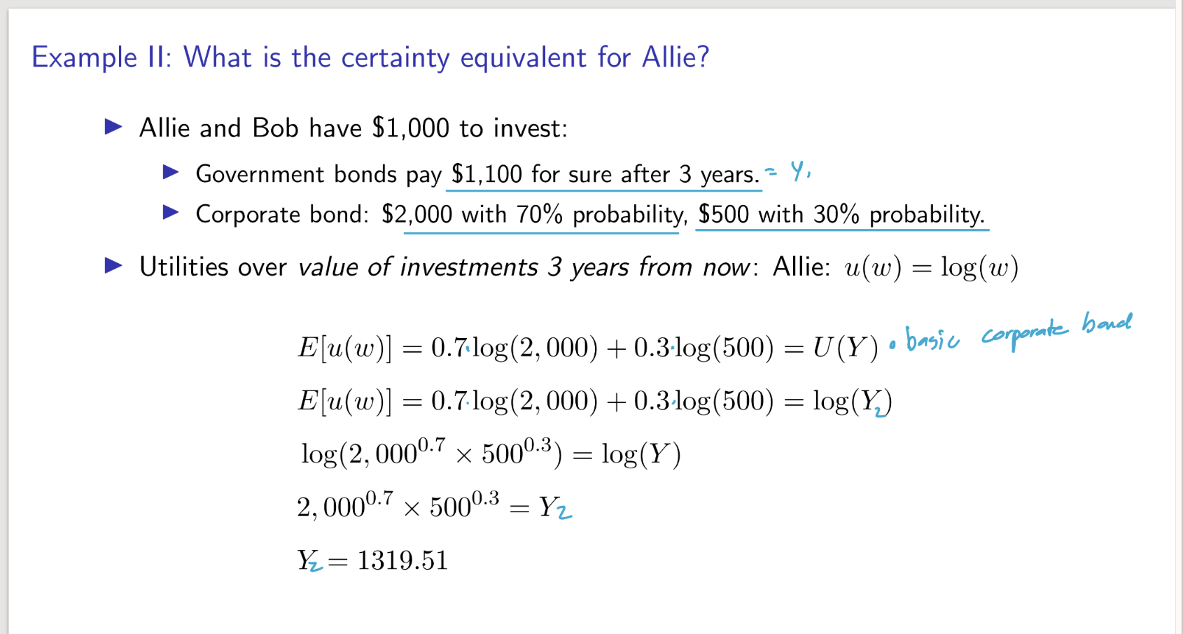
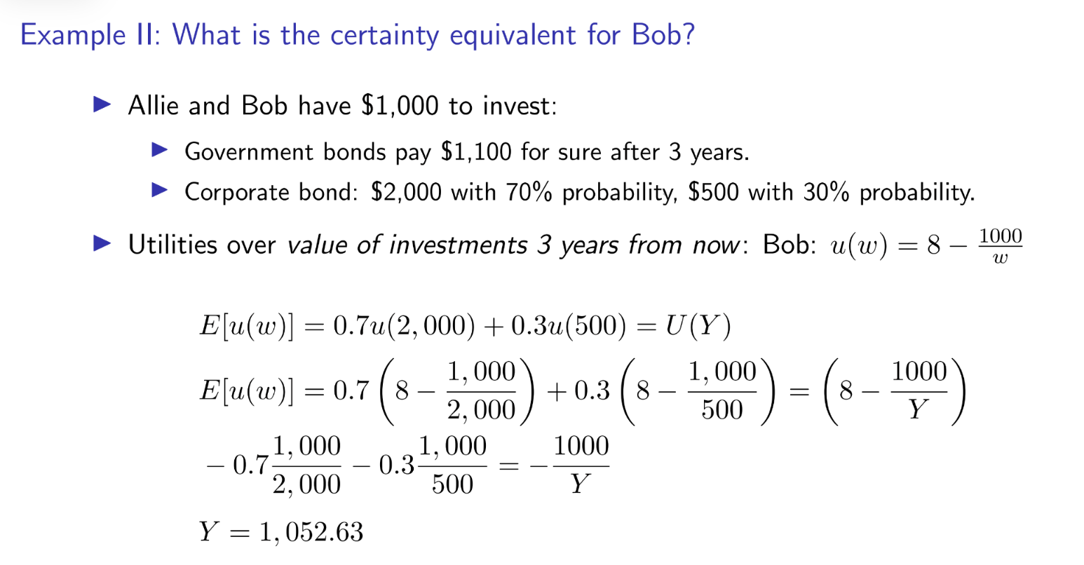
Certainty Equivalent

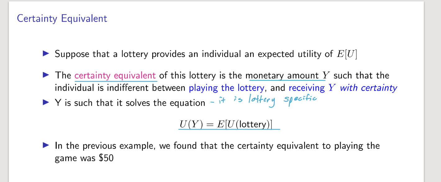
• basically how we solve for m by making the utility = function and solving for x

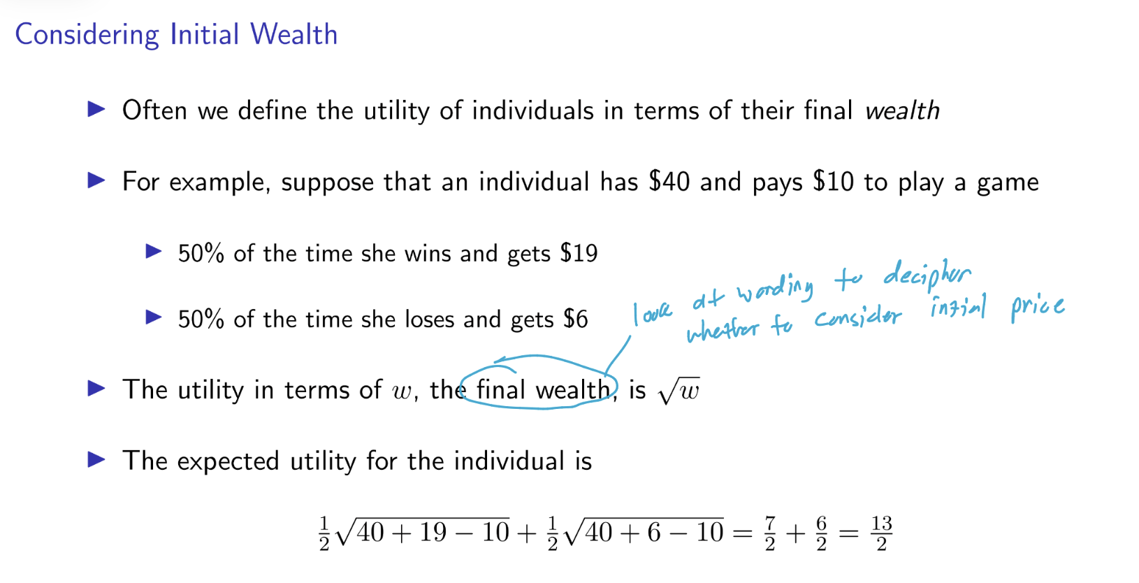
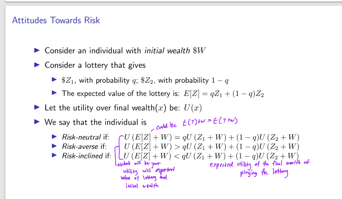
Considering Initial Wealth

Bob and Allie Risk Aversion

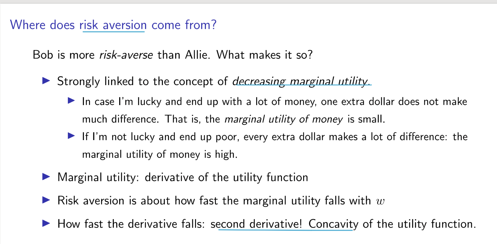
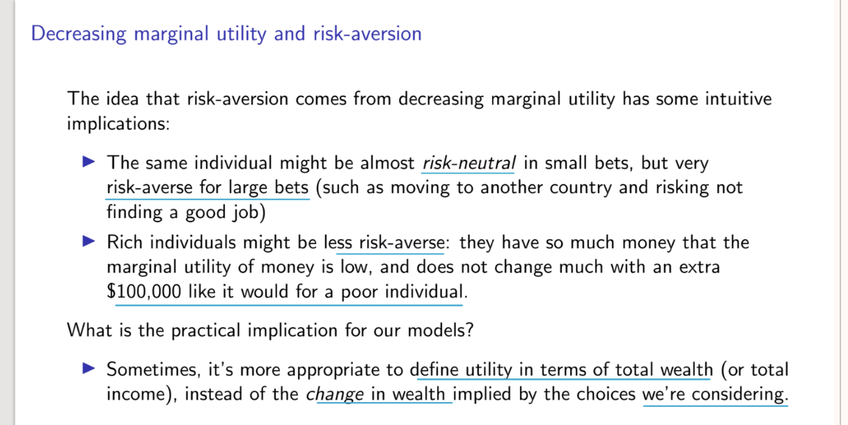
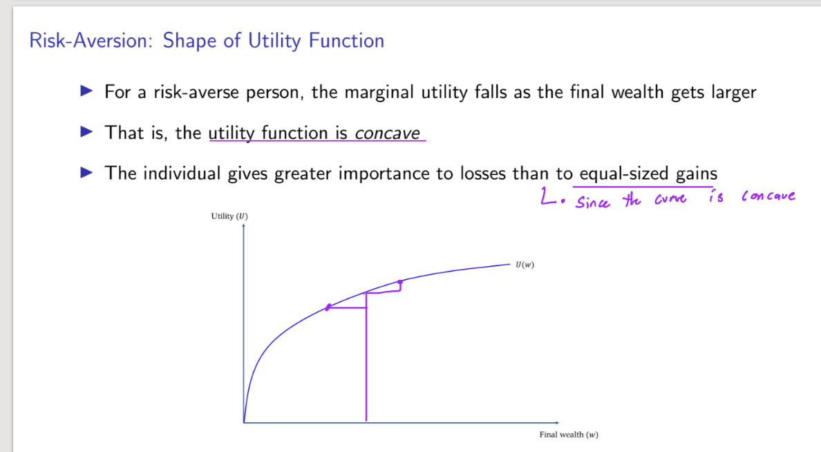
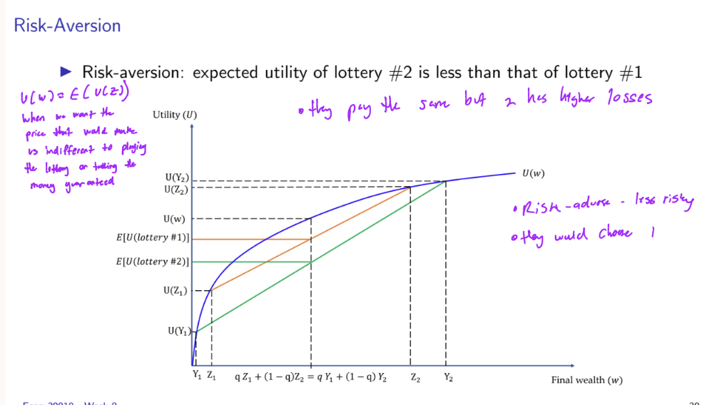
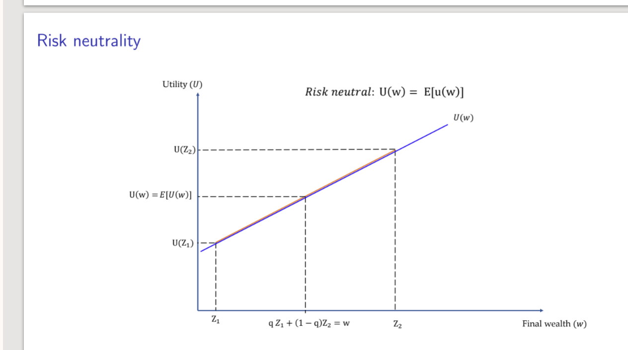
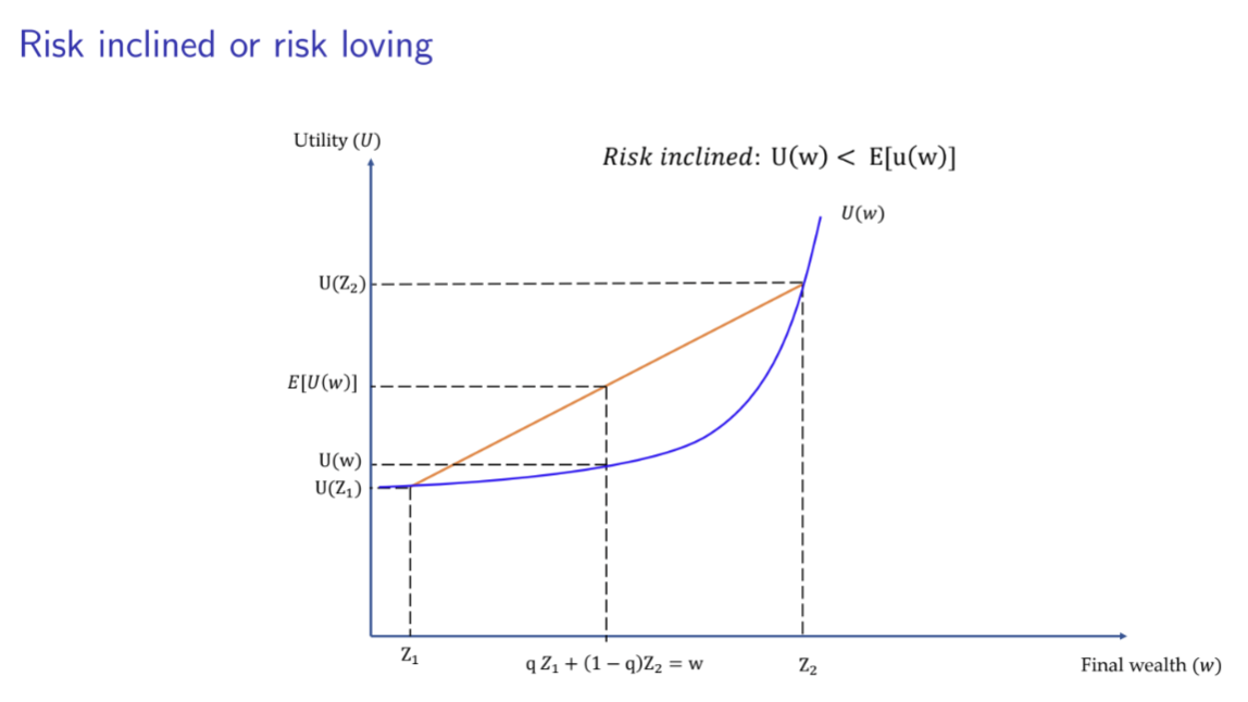
• the second derivative of utility tells us if a person is risk inclined, risk adverse, or risk neutral. → below 0 → diminishing marginal utility and risk adverse(concave “frowns”) & equal to 0 → constant marginal utility and risk neutral and above 0 → means increasing marginal utility and risk inclined

Attitude Towards Risk and Deciphering what type of risk they’d take on

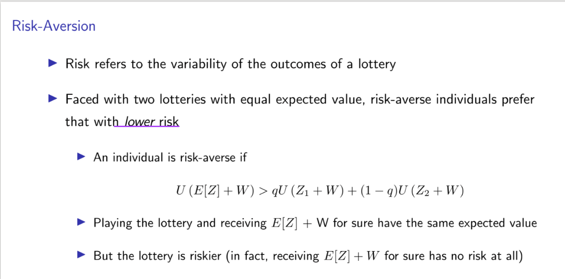
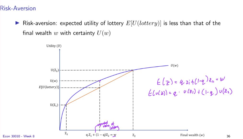
Risk Aversion

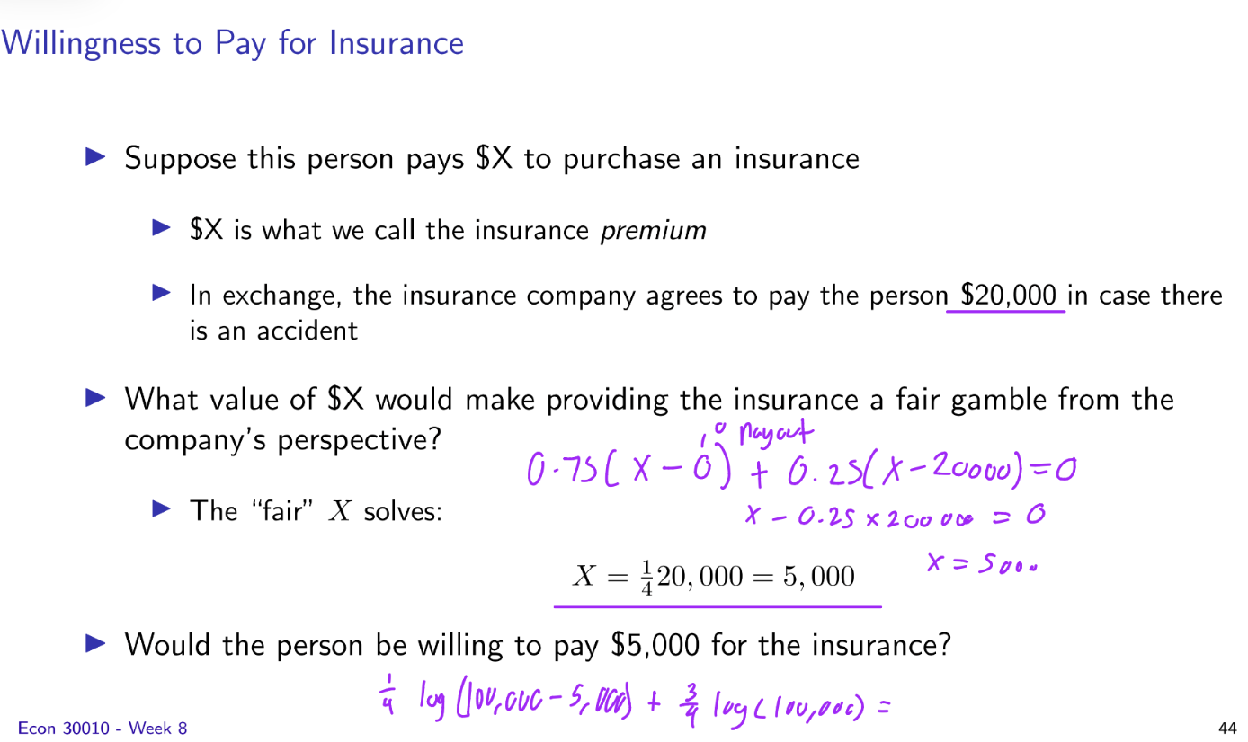
Insurance - what insurance premium makes a fair gamble from company perspective?

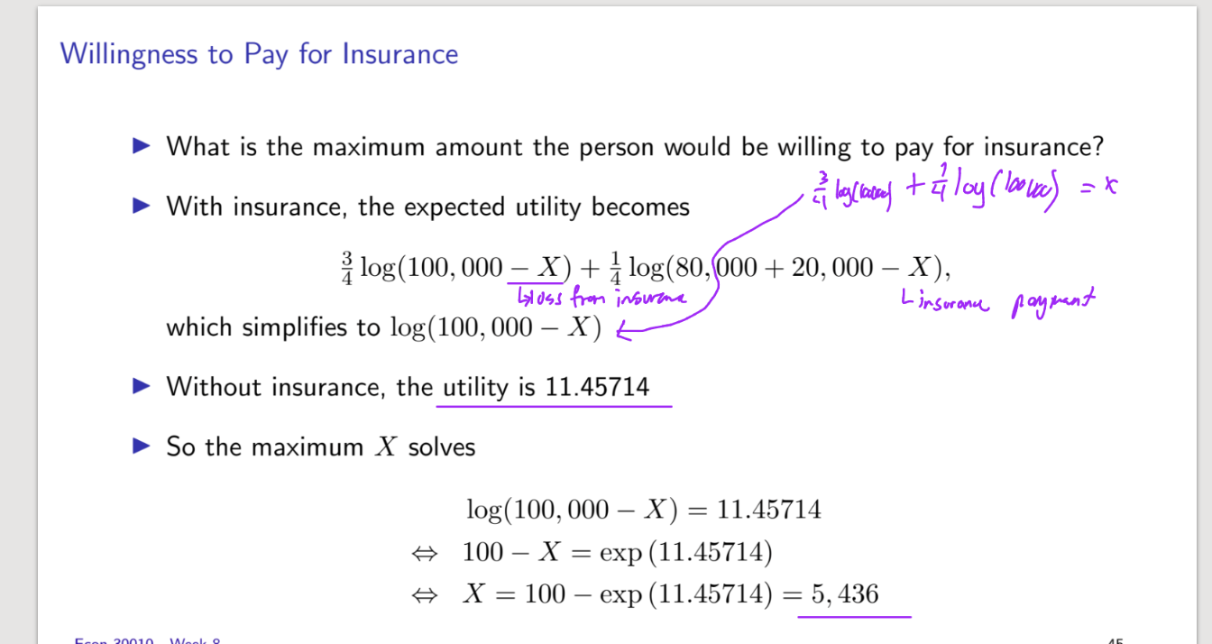
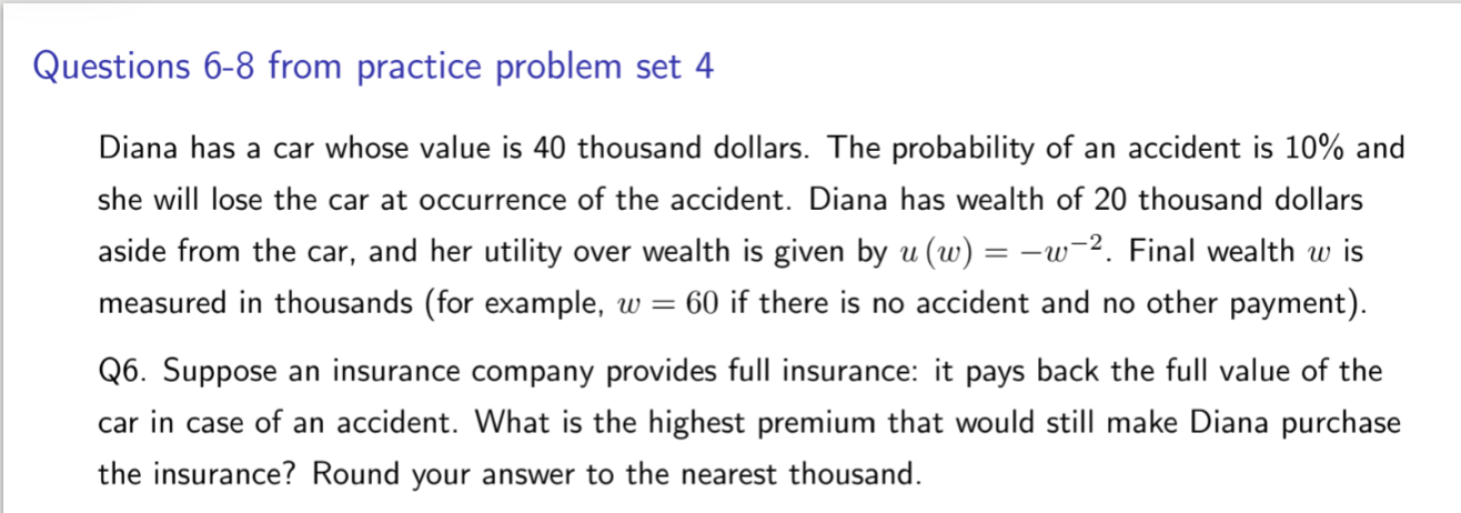
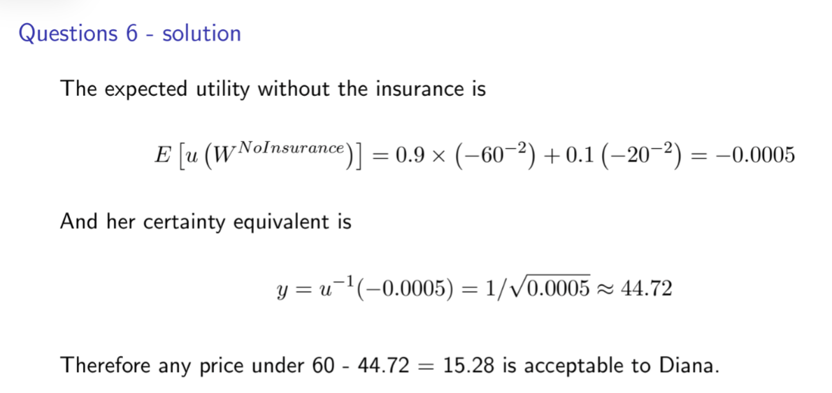
Max someone would spend on insurance

Uncertainty + Certainty Equivalent + Different risks Summary

Risk Neutrality Graph

Risk-inclined or risk-loving graph

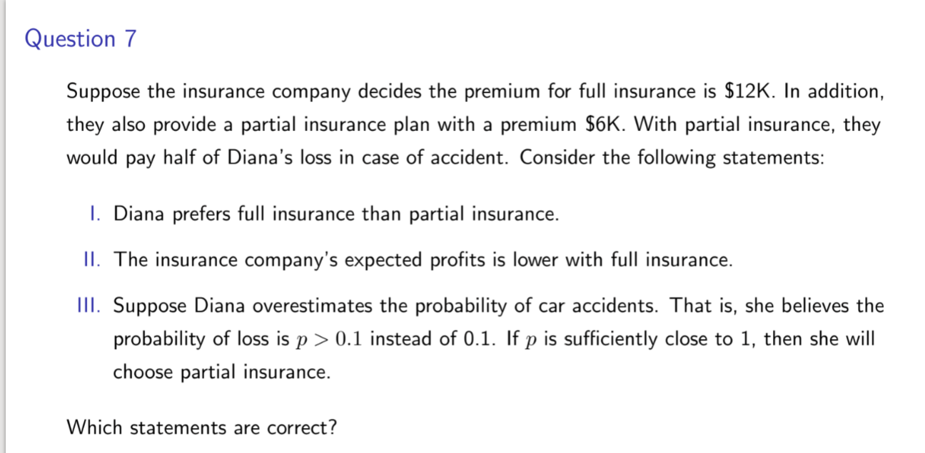
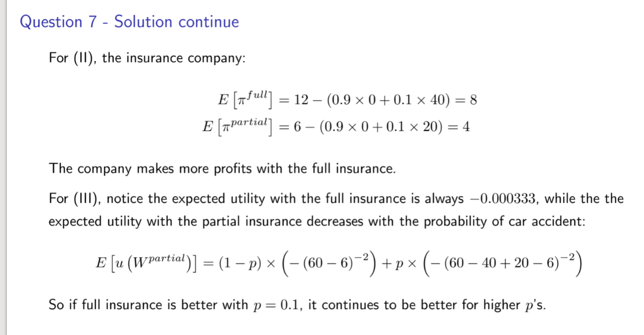
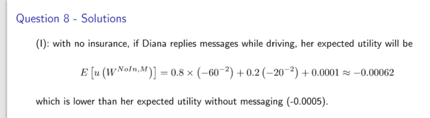
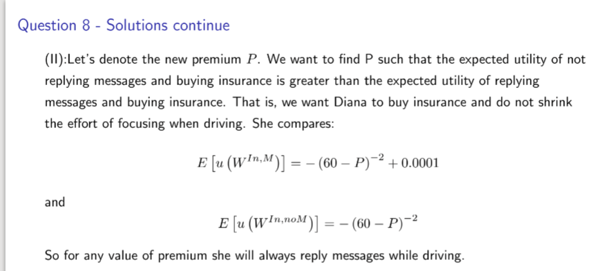
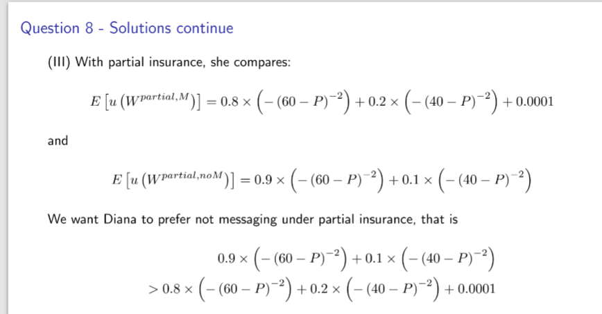
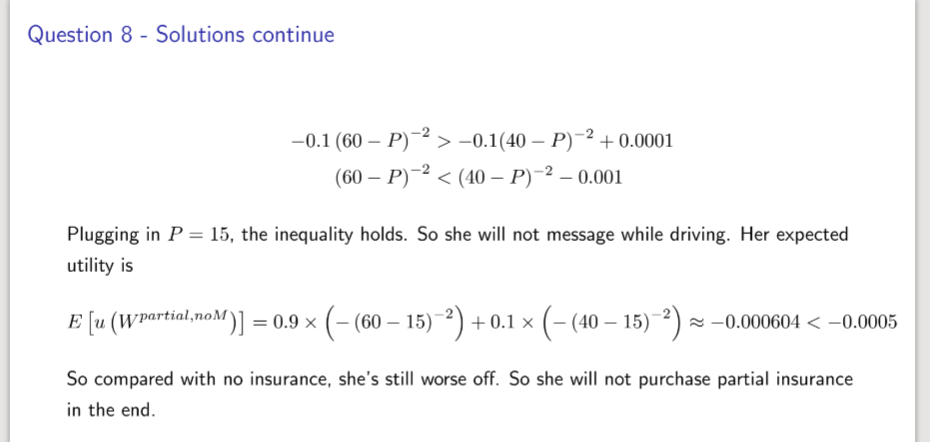
Diana

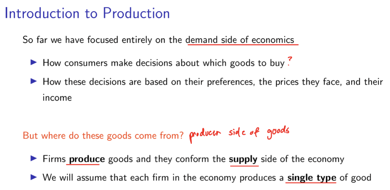
Introduction to Production

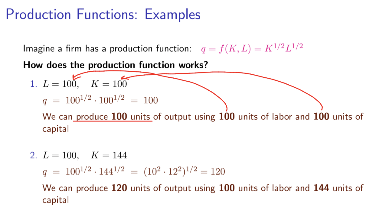
Production Functions

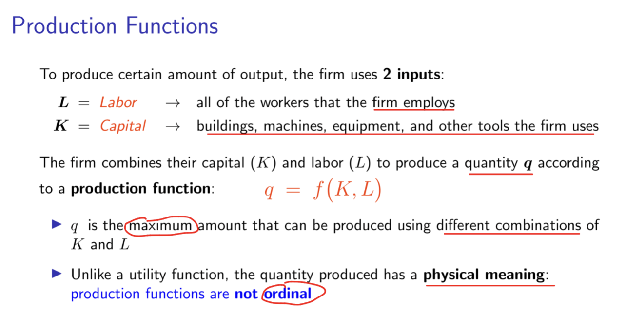
• production functions are not ordinal → meaning they’re the output number q has a specific physical meaning that can be measured and compared in absolute terms.

Marginal Physical Product