calc3 :::::::))))))))))))))))))))) love and happiness and sparkles and yayayayayay

yayayayayay dontfail yayayayyaya

cos²(θ)+sin²(θ)=

1

1+tan²θ=

sec²θ

I+cot²θ=

csc²θ

sinθ/cosθ=

tanθ

cosθ/sinθ=

cotθ

1/cosθ=

secθ

1/sinθ=

cscθ

d/dx (f(x)g(x)) =

f(x)g’(x) + f’(x)g(x)

d/dx(f(x)/g(x)) =

g(x)f’(x) - f(x)g’(x) / (g(x))²

d/dx (f(g(x))) =

f’(g(x))g’(x)

d/dx (e^x) =

e^x

d/dx (ln(x)) =

1/x

d/dx (sin(x)) =

cos(x)

d/dx ( cos(x)) =

-sin(x)

d/dx (tan(x)) =

sec²(x)

d/dx (sec(x)) =

sec(x)tan(x)

d/dx (csc(x)) =

-csc(x)cot(x)

d/dx (cot(x)) =

-csc²(x)

d/dx (arcsin(x)) =

1/root(1-x²)

d/dx (arccos(x)) =

-1/root(1-x²)

d/dx (arctan(x)) =

1/(1+x²)

a dot b =

magnitude(a)*magnitude(b)*cosθ, where θ is the angle between the vectors a and b

a cross b =

magnitude(a)*magnitude(b)*sinθ, where θ is the angle between the vectors a and b

proj_ab =

((a dot b)/(a dot a))*a

The distance D from a point P₁ to a line l with direction vector L is given by

D = magnitude(L cross (P₀-P₁) / magnitude(L), where P₀ is any point on the line l

Given a vector-valued function with a parametrization r(t): R → R³, we can define the Frenet frame:

• T(t) = (r’(t)/magnitude(r’(t)))

• N(t) = (T’(t)/magnitude(T’(t)))

• B(t) = T(t) cross N(t)

The arc length function for a curve parametrized by r(t): R → R³ is

s(t) = integral from 0 to t of magnitude(r’(t) *dt

The tangential and normal componenets of acceleration are given by

• a(t) = a_T(t)T(t) + a_N(t)N(t)

• a_T(t) = d/dt * magnitude(r’(t))

• a_N(t) = magnitude(r’(t))*magnitude(dT/dt)

The second derivative test for unconstrained optimization

Suppose that (x,y) is a critical point of f(x,y) (which is a point such that f_x(x,y) = 0 and f_y(x,y) = 0). At the critical point, compute the quantity D(x,y) = f_xx(x,y)f_yy(x,y) - [f_xy(x,y)]².

• If D>0 and f_xx(x,y)>0, then (x,y) is a local minimum

• If D>0 and f_xx(x,y)<0, then (x,y) is a local maximum

• If D<0, then (x,y) is a saddle point

• If D = 0, the test is inconclusive

The method of Lagrange multipliers for constrained optimization

To optimize f(x,y) subject to a constraint g(x,y) = c for some constant c, find all critical points tot he constrained optimization problem as solutions to the system: gradient(f(x,y)) = lambda*(gradient(g(x,y))), g(x,y) = c, for a real number lambda called a Lagrange multiplier.

Surface area of the graph of z = f(x,y) above the region R in the xy plane is

A = (double integral over R) root(1 + magnitude(gradient f(x,y))²)dA = (double integral over R) root(1+ [f_x(x,y)]² + [f_y(x,y)]²)dA

polar coordinates

x = rcosθ

y = rsinθ

dA = rdrdθ

cylindrical coordinates

• x = rcosθ

• y = rsinθ

• z = z

• dV = rdzdrdθ

spherical coordinates

• x = rho sin(phi)cosθ

• y = rho sin(phi)sinθ

• z = rho cose(phi)

• tan(phi) = r/z

• dV = rho²sin(phi)d(rho)d(phi)dθ

Change of variables: jacobian, formula

• jacobian: d(x,y)/d(u,v) = (dx/du)(dy/dv) - (dx/dv)(dy/dv)

• change of variables: double integral over R of f(x,y)dxdy = double integral over R’ of f(u,v) (ABS VAL OF d(x,y)/d(u,v)) dudv, where R’ is the region R transformed to (u,v) variables and f(u,v)= f(x(u,v), y(u,v))

tangential component of acceleration using velocity

a_T(t) = (v dot a) / magnitude(v)

how to find an equation of the plane containing points 1, 2, 3

• p2-p1 = v1

• p3-p2 = v2

• normal vector = v1 cross v2, result ijk are your xyz coefficients

• then plug any one of your original points in to that expression to find the right-hand side scalar

how to show that a line is parallel to a plane

dot product must be 0

how to find distance from line to plane

line equation: (point) + t

cos²(pi/4)=

1/2u

v and w are perpendicular if

v dot w = 0how

how to know if two planes are parallel

two planes are parallel if their normal vectors are scalar multiples of one another

how to determine the symmetric equation of a line containing a point and parallel to both of the planes.

To be parallel to both planes, the line must be perpendicular to both normal vectors → cross product

• result are your abc denominators

• numerators are x-x_0, y-y₀, z-z₀

sphere standard form

(x-h)²+(y-k)²+(z-l)²=R²

how to complete the square

take half of b and square it, add to both sides

how to find the points where a curve intersects a sphere

• sub in x=i, y=j, z=k of the parametrization to the sphere equation

• solve for t and plug back into parametrization to find a specific point

how to find r(t) from v(t)

r(t) = integral of v(t)

Equation of a tangent plane

F_x(x₀,y₀,z₀)(x-x₀)+F_y(x₀,y₀,z₀)(y-y₀)+F_z(x₀,y₀,z₀)=0

directional derivative

D_vf= gradient of f dot u

• where u is just the unit vector of whatever direction vector is given

Distance between point P₁ and a plane

• find the normal vector of the plane, dot w P₁-P₀, abs val of that

• divide by magnitude of normal vector

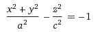
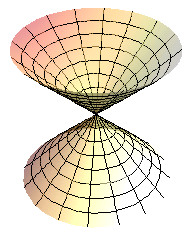
hyperboloid of two sheets (surface)

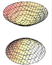
hyperboloid of two sheets (equation)

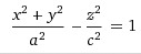
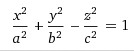
one‐sheeted hyperboloid (Surface)

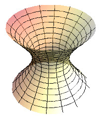
one‐sheeted hyperboloid (Equation)

paraboloid (surface)

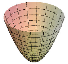
paraboloid (equation)

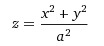
cone (surface)

cone (equation)

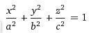
ellipsoid (surface)

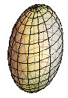
ellipsoid (equation)

one-sheeted elliptical hyperboloid (surface)

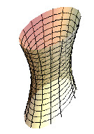
one-sheeted elliptical hyperboloid (equation)

hyperbolic paraboloid (surface)

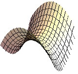
hyperbolic paraboloid (equation)

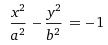
hyperbolic cylinder (surface)

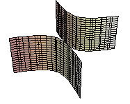
hyperbolic cylinder (equation)

elliptic cylinder (equation)

(x/a)² + (y/b)² = 1

arc length formula

L([a, b]) = integral from a to b of the magnitude of r’(t) dt

d/dx(integral from 1 to x² of e^t dt) =

e^x²(2x)

direction of maximal increase/decrease

max increase = gradient f

max decrease = - gradient f

max rate of increase/decrease

max rate of increase = magnitude of gradient f

max rate of decrease = - (magnitude of gradient f)

how to find the point with the smallest x-coordinate w constraint

f(x,y) = x bc thats what you’re optimizing, g(x,y) = constraint equation

gradient f = lambda gradient g, from there form your two equations (including constraint)

solve for x,y to find CP (case 1, case 2, etc) and see which option optimizes (in this case, where x is smallest)

jacobian

abs val of det[ dx/u dxdv ; dy/du dydv]

divF, and the result is what type?

divF = F dot del, always a scalar

curlF, and the result is what type?

curlF = F cross del, always a vector

line equation in vector form

r(t) = (x₀, y₀, z₀) + t(a, b, c)

line equation in parametric form

x(t) = x₀+at, y(t) = y₀+bt, z(t) = z₀+ct

line equation in symmetric form

(x-x₀)/a = (y-y₀)/b = (z-z₀)/c

plane equation

ax+by+cz = d

vector valued function def

function r that inputs a real # (parameter) t and outputs a vector/point in Rⁿ

how to know if a curve is smooth

a curve is smooth if r(t) is continuous and the magnitude of r’(t) DOES NOT equal 0 for all t

how to know if a curve is PIECEWISE smooth

parametrization is piecewise smooth if the interval is composed of subintervals on each of which r is smooth

Frenet frame meaning

• T(t) = unit tangent - directional steepness

• N(t) = unit normal - curvature/bending

• B(t) = unit binormal - lifting off from a plane

how to find level surface/curve

set vars = 0 and solve

• surface = 3D, curve = 2D

minimize/maximize the distance subject to contraint g…

f(x,y) = x²+y² (distance: really this optimizes D² but the points are the same as optimizing D, so this is easier)

volume/area integrals

volume: triple integral over v of 1 dV

area: double integral over R of 1 dA

iterated integral def

integrating with respect to one variable while holding others constant

surface area formula

A = double integral over R of root(1+(magnitude of gradient f)²) dA

change of variables

double integral over R of f(x,y)dA = double integral over S of f(g(u,v))*abs value of jacobian dA

Stokes’ Theorem

single integral over C of F dot dr = double integral over sigma of (curlF dot n dS)

• use whenever you see curl in the question → immediately stokes

Green’s theorem (sigma is flat)

single integral over C of (M dx+Ndy) = double integral over R of (dN/dx - dM/dy)dA

• use whenever you see two things dx and dy being added

Fundamental Theorem of Line Integrals

single integral over C of (delF dot dr) = f(end)) - f(start)

• where f is the potential function

divergence theorem

double integral over sigma of (F dot n dS) = triple integral over D of (divF dV) for outward n (- if opposite orientation)

line integral

single integral over gamma of (f dS) = single integral from a to b of (f(r(t))*magnitude of r’(t) dt)

when calculating line integrals order of thinking

1. Is there a potential function? Calculate curlF to see if = 0 and/or just determine potential function by inspection

2. then plug in end point and start point to potential function → end-start

Green’s Theorem

single integral over gamma of (Pdx + Qdy) = double integral over D of (dQ/dx - dP/dy)dA

• if gamma is counterclockwise, you’re good

• if gamma is clockwise, *-1

When to use Green’s Theorem

• if the line is tracing out a closed, easy shape (circle, semicircle, triangle, square, etc)

volume of sphere :(

4/3 pi r³

stokes steps

1. name curl and apply stokes formula (double integral over sigma of curlf dot n dS

2. parametrize the line integral and solve