Probability Distributions and Key Concepts in Statistics

Discrete Uniform E[X]

(n+1)/2

Discrete Uniform Var[X]

(n^2-1)/12

Binomial

Counts the number of successes in n independent Bernoulli trials, each with the same probability of success p.

Binomial Example

a. Flipping a coin n times and counting the number of heads

Binomial P(X=x)

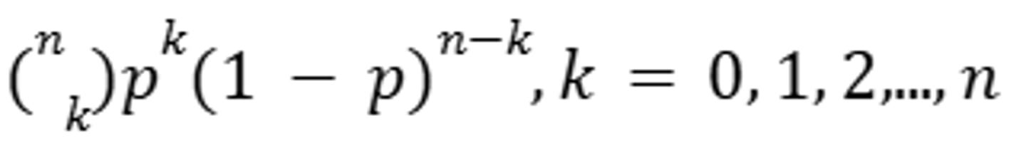
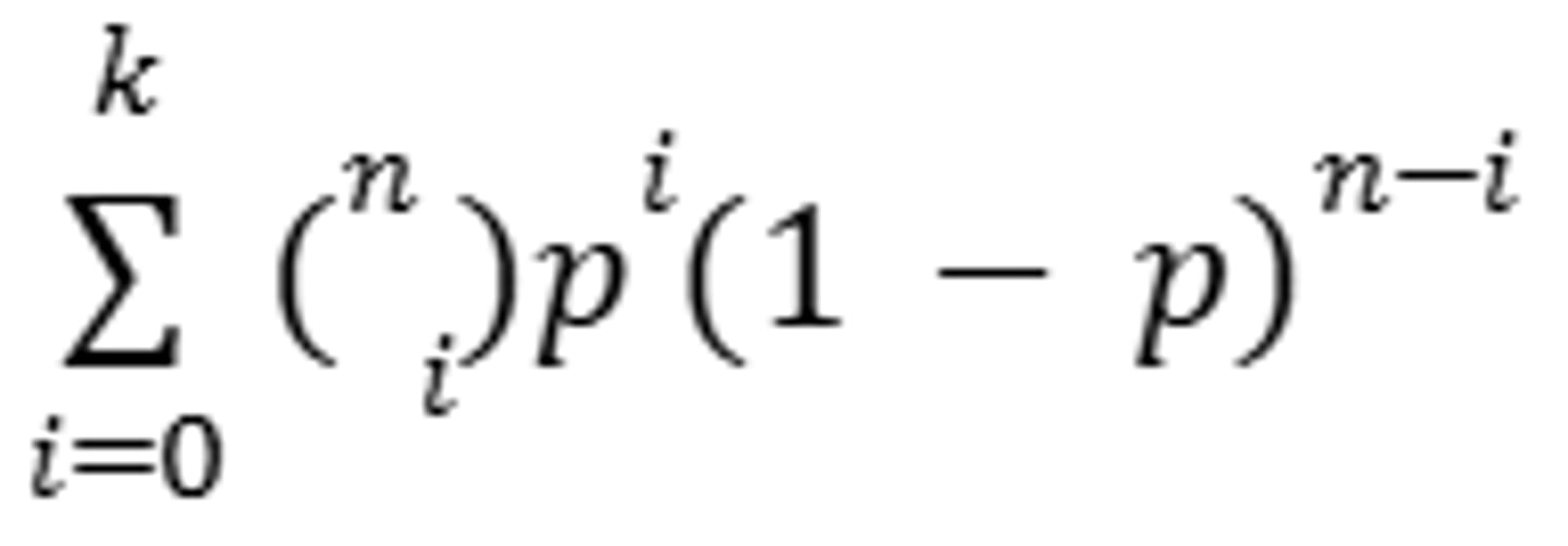
Binomial P(X<=x)

Binomial E[X]

np

Binomial Var[X]

npq

Geometric

The number of independent Bernoulli trials needed to get the first success, where each trial has the same probability of success p

Geometric Example

Shooting hops until you make a three-point shot

Discrete Uniform

A discrete uniform r.v. is one where all outcomes are equally likely

Discrete Uniform Examples

a. Flipping a coin n times and counting the number of heads

b. Number of defective items in a batch of n products

Discrete Uniform P(X=x)

1/n

Discrete Uniform P(X<=X)

x/n, 1<=x

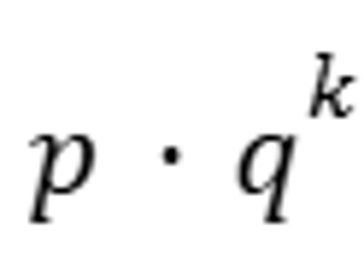
Geometric Pr(X=k)

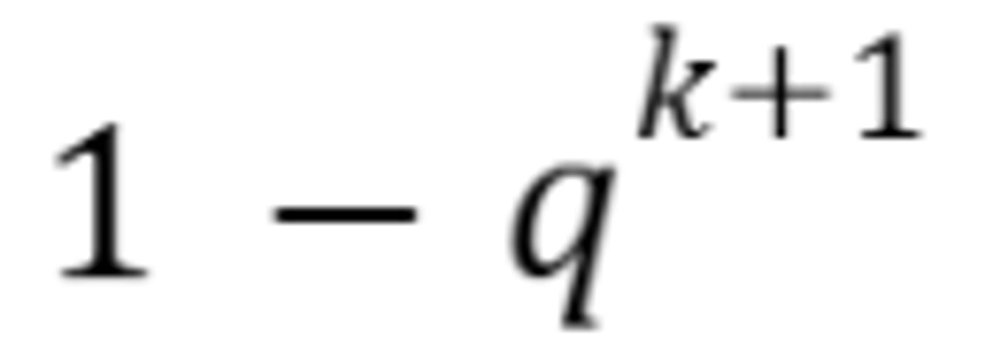
Geometric Pr(X<=k)

Geometric E[X]

q/p

Geometric Var[X]

q/p^2

Negative Binomial

Generalization of the geometric distribution

Negative Binomial Example

Number of missed free-throws before the 10th success

Negative Binomial Pr(M=k)

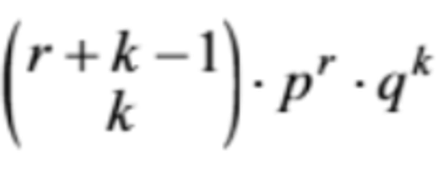
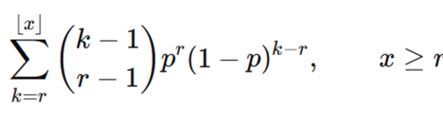
Negative Binomial Pr(M<=k)

Negative Binomial E[X]

rq/p

Negative Binomial Var[X]

rq/p^2

Hyper-geometric

The number of successes in a sample of size n drawn without replacement from a finite population of size n that contains exactly G good outcomes and B bad outcomes.

Hyper-geometric Example

Drawing cards from a deck without replacement

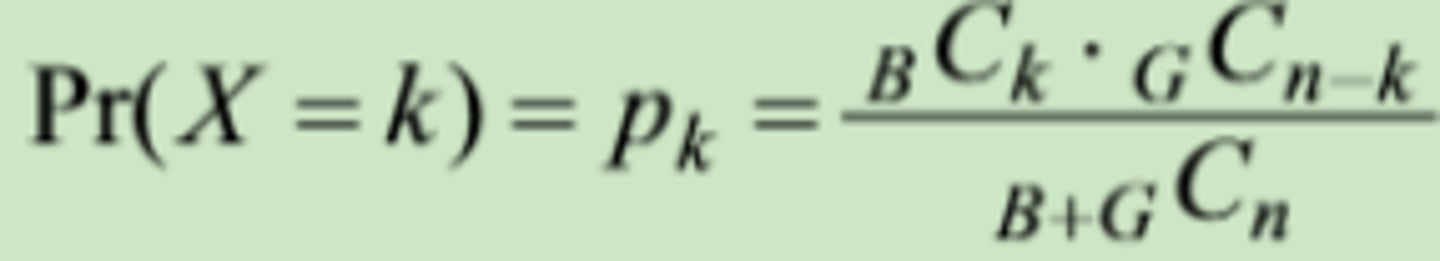
Hyper-geometric Pr(X=x)

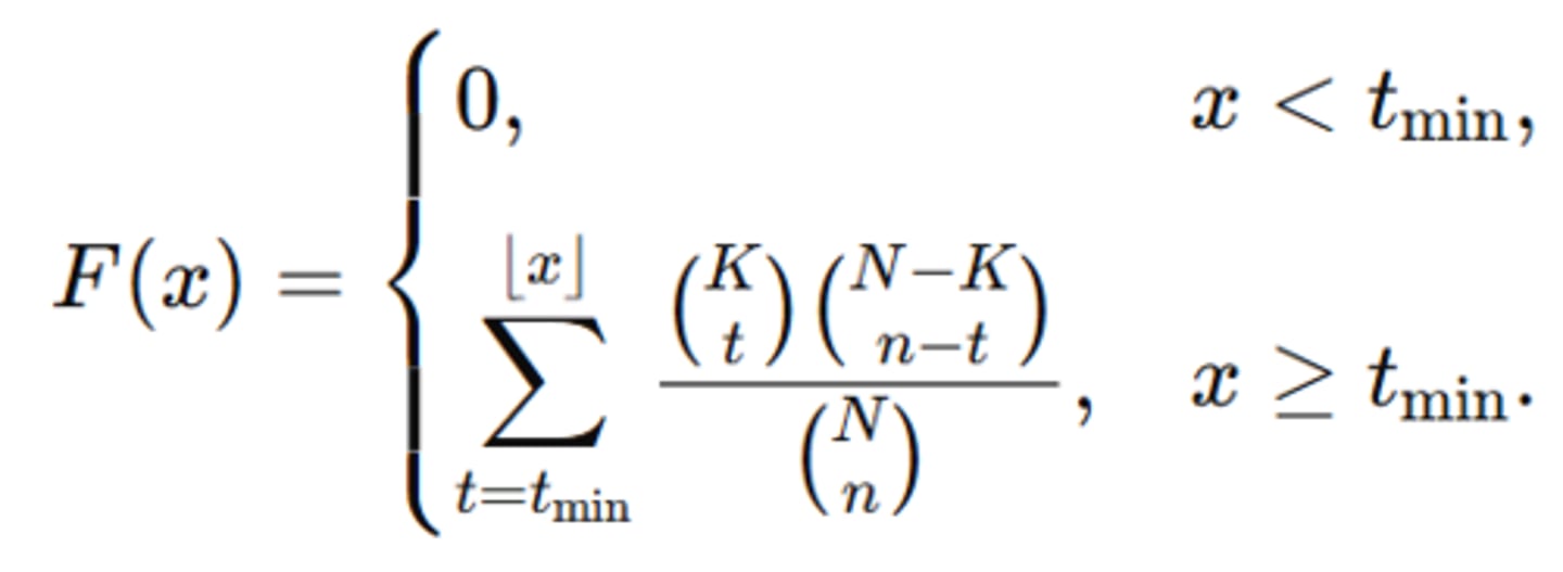
Hyper-geometric Pr(X<=x)

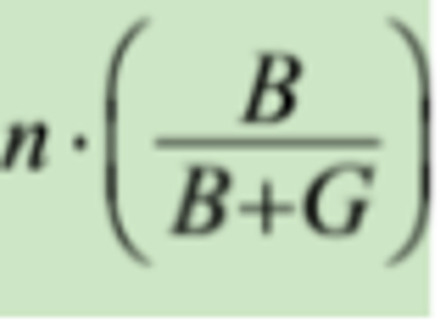
Hyper-geometric E[X]

Poisson

Used to count the number of times a random and sporadically occurring phenomenon actually occurs over a period of observation.

Poisson Examples

Misprints in a manuscript

Phone calls coming into a call-service center

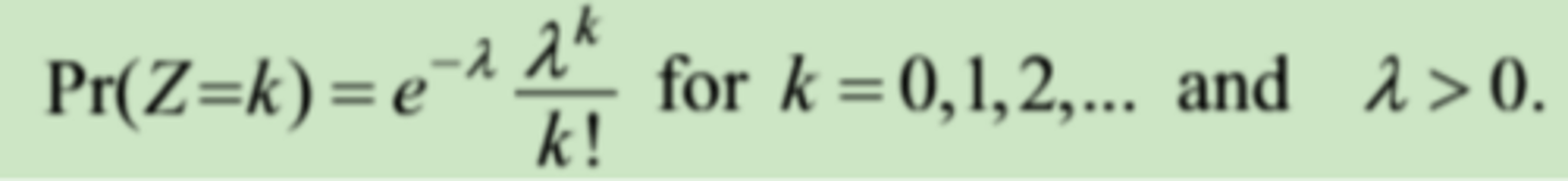
Poisson Pr(X=k)

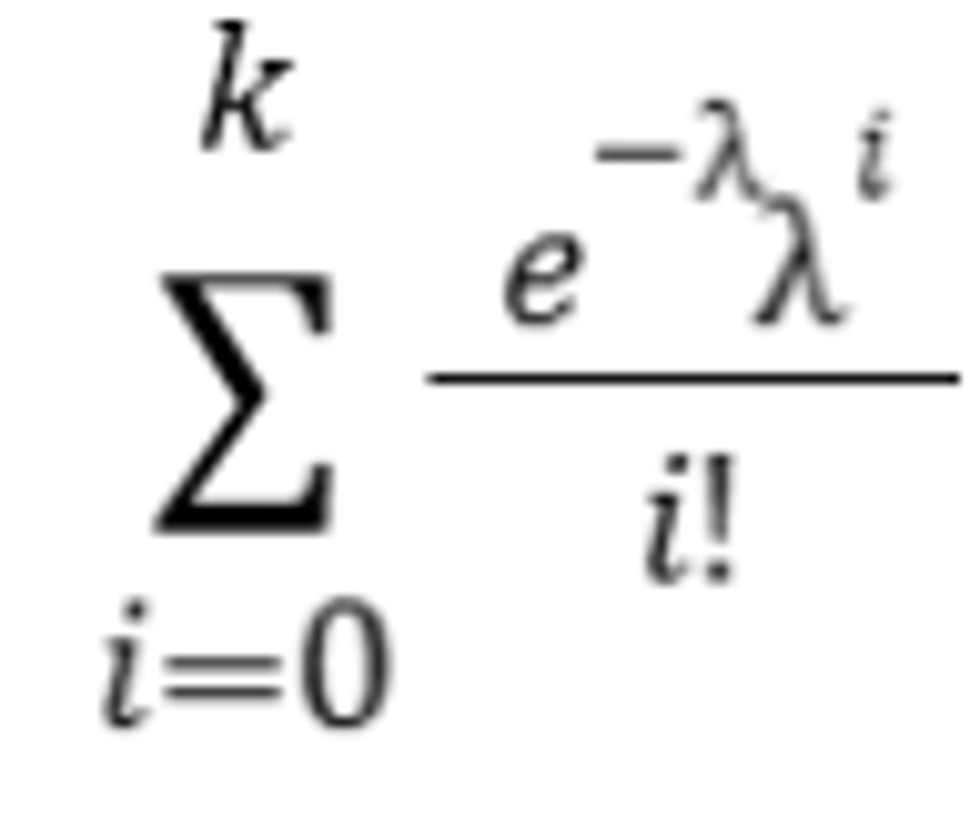
Poisson Pr(X<=k)

Poisson E[X]

λ

Poisson Var(X) =

λ

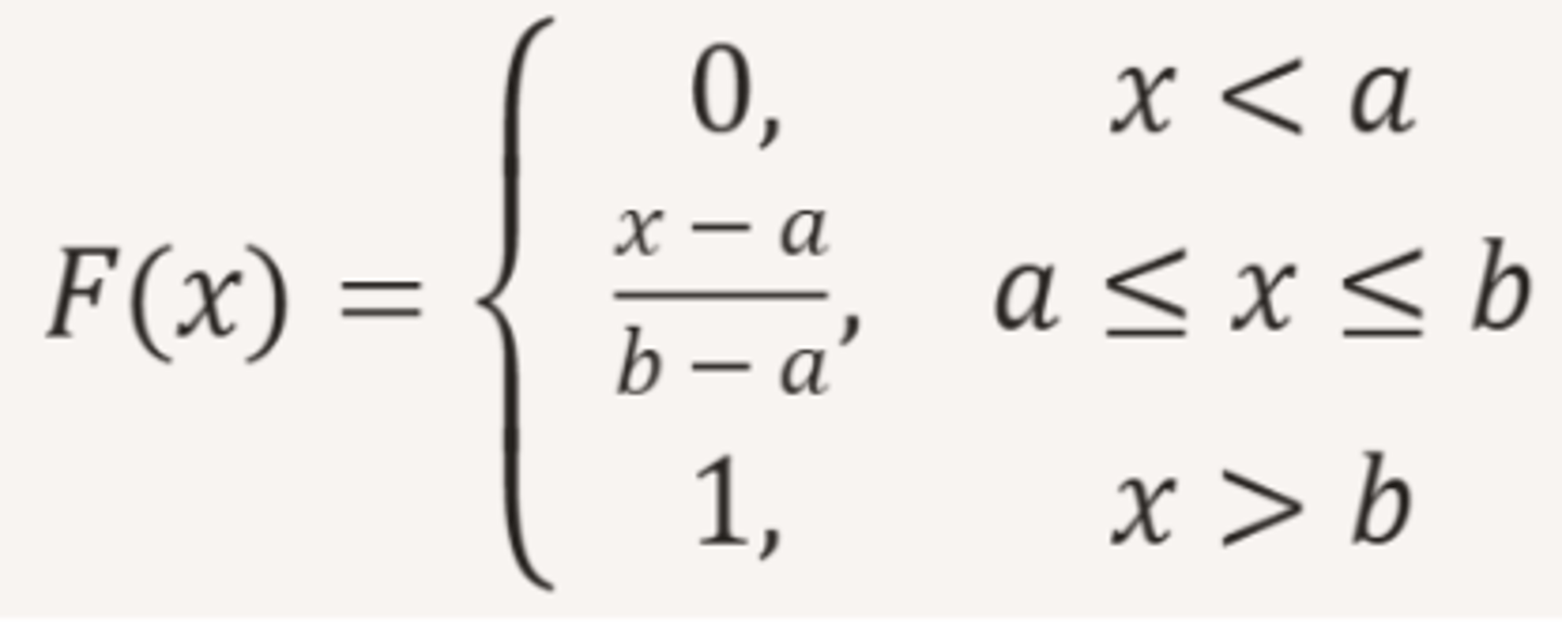
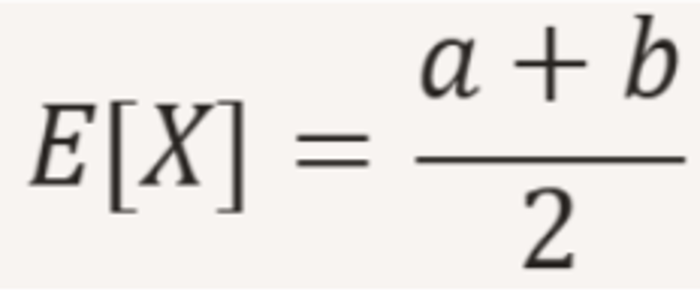
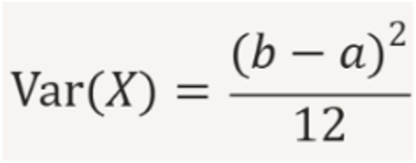
Continuous Uniform

A continuous uniform random variable models a situation where every value in an interval is equally likely.

Continuous Uniform Examples

A bus arrival time uniformly distributed between 0 and 10 minutes

A random point chosen along a 2‑meter stick

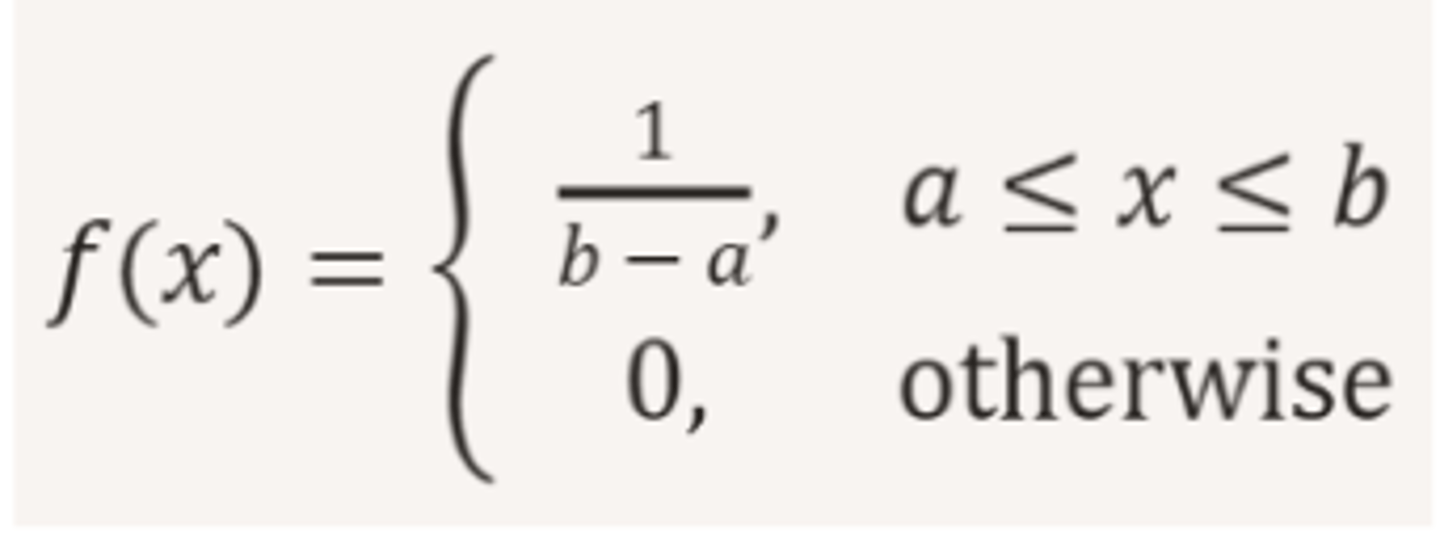
Continuous Uniform f(x)

Continuous Uniform F(x)

Continuous Uniform E[X]

Continuous Uniform Var[X]

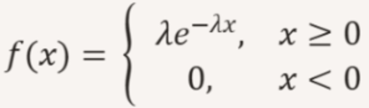
Exponential

The exponential distribution models waiting times between independent events that occur at a constant average rate.

Exponential Examples

Time between customer arrivals at a service counter

Time until a radioactive particle decays

Exponential f(x)

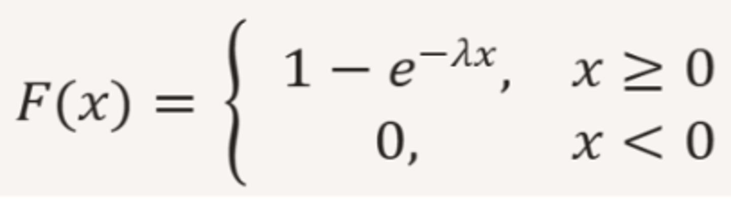
Exponential F(x)

Exponential E[X]

1/λ

Exponential Var[X]

1/λ^2

Standard Normal

Models standardized measurements that arise from many small, independent sources of variation.

Standard Normal Examples

Standardized test scores (after converting to z‑scores)

Measurement errors in engineering and physics

Heights, weights, and biological traits (after standardization)

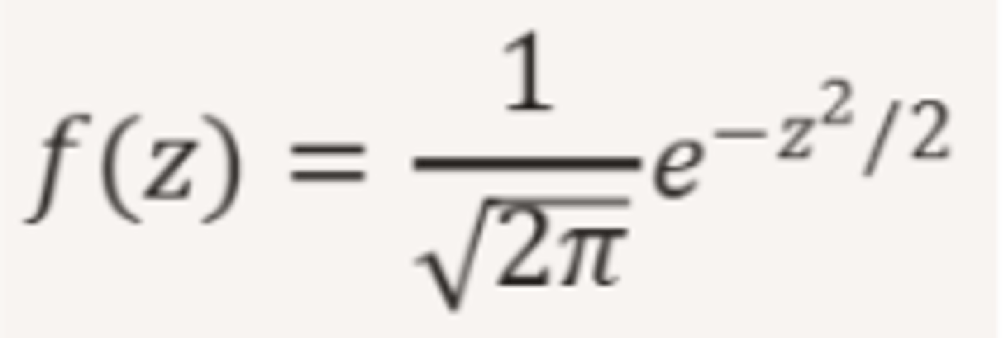
Standard Normal f(x)

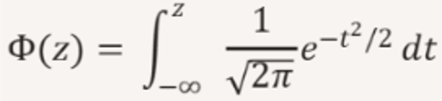
Standard Normal F(x)

Standard Normal E[X]

0

Standard Normal Var[X]

1

General Normal

The general normal distribution models continuous quantities influenced by many small, independent sources of variation.

General Normal Examples

Human traits such as height, weight, reaction time

Aggregated measurement errors

General Normal f(x)

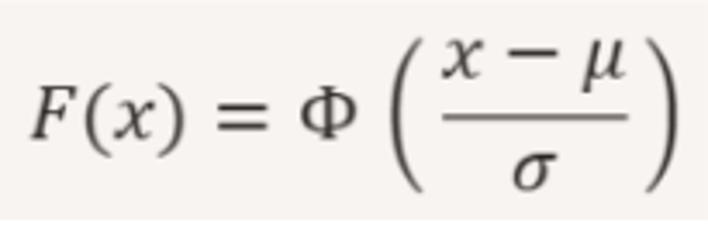
General Normal F(x)

General Normal E[x]

µ

General Normal Var[x]

σ^2

Lognormal

Models positive‑valued quantities whose logarithm is normally distributed. It naturally appears when a process involves multiplicative effects rather than additive ones.

Lognormal Examples

Component lifetimes in reliability engineering

Time‑to‑failure for mechanical systems with multiplicative degradation

Income distributions and wealth models

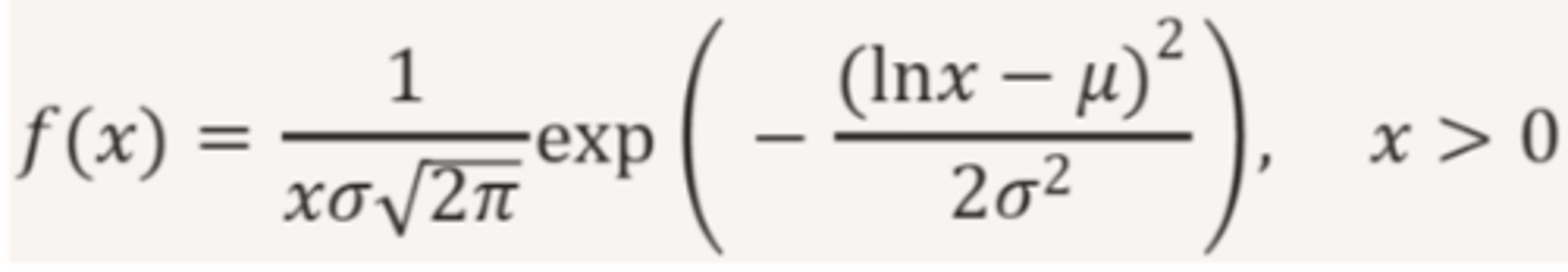
Lognormal f(x)

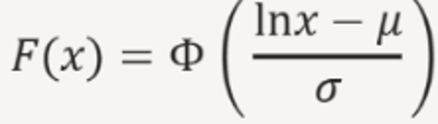
Lognormal F(x)

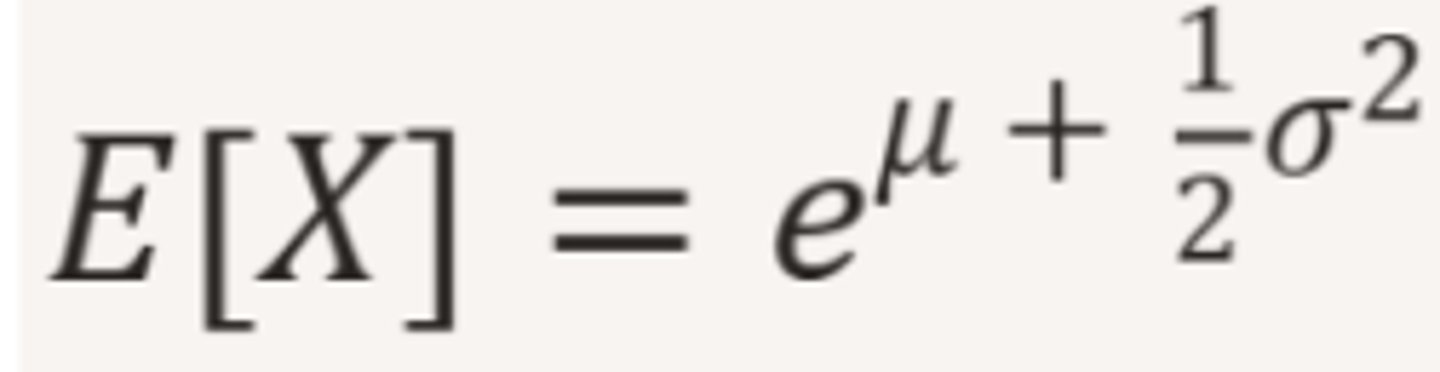
Lognormal E[X]

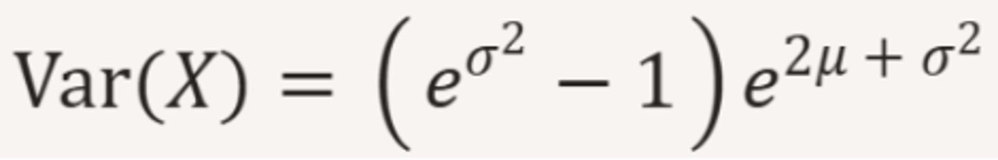
Lognormal Var(X)

Gamma

Models positive‑valued quantities that accumulate through additive waiting times.

Gamma Examples

Total time until the k‑th failure in reliability engineering

Lifetimes of components with multiple sequential degradation stages

Rainfall amounts and hydrology modeling

Gamma f(x)

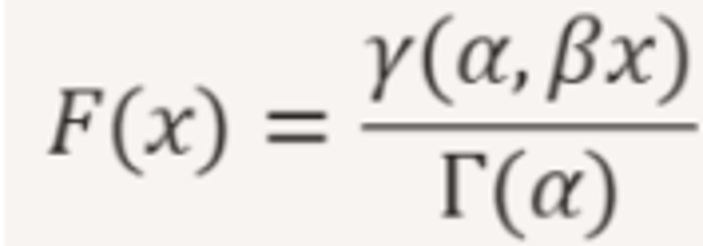
Gamma F(X)

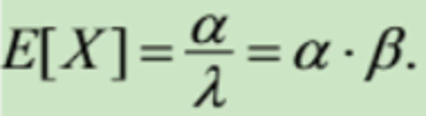
Gamma E[X]

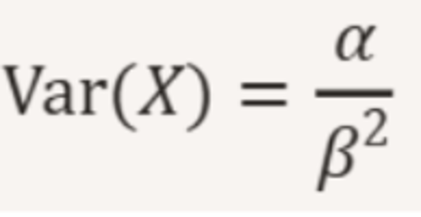
Gamma Var[X]

Beta

Models quantities constrained to the interval [0,1].

Beta Examples

Reliability: modeling component success probabilities

Random variables representing fractions (e.g., proportion of time a system is operational)

Modeling bounded physical quantities (e.g., porosity, humidity, mixture ratios)

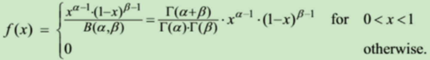
Beta f(x)

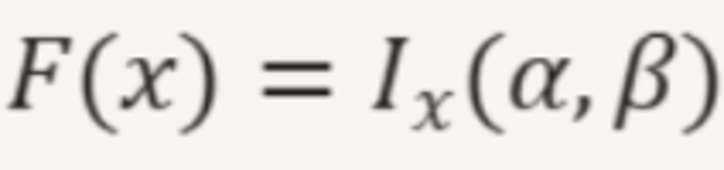
Beta F(X)

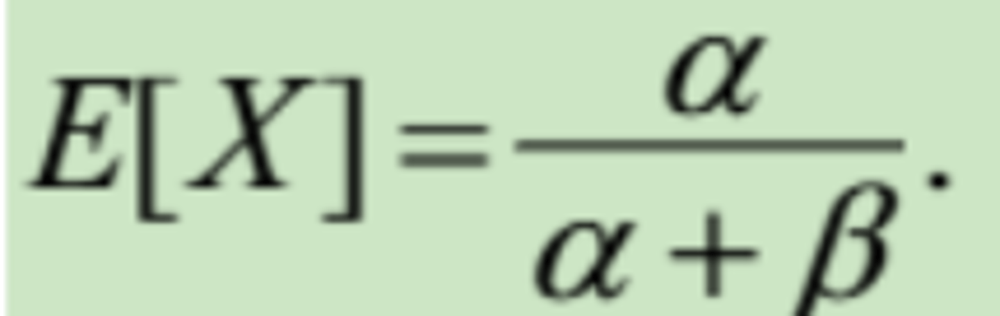
Beta E[X]

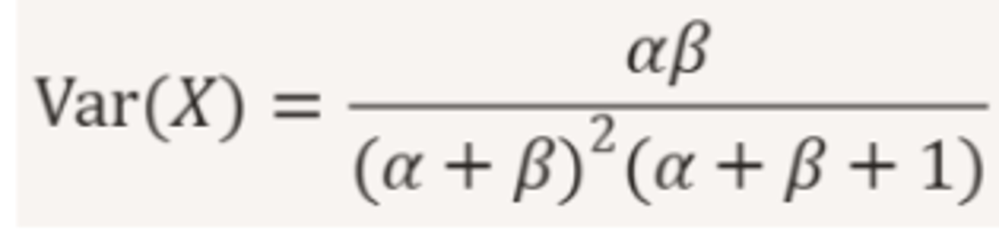
Beta Var(X)

Still learning (10)

You've started learning these terms. Keep it up!