data analysis midterm

how to identify research questions

specific events → general patterns (greater applicability)

hypothesis

theory-based statement about what we would expect to observe if our theory is correct

how to develop theories

examine previous research on the topic

• what other causes of DV did previous research miss

• can their theory be applied elsewhere

hypothesis testing

1. measurement of variables

2. data collection

3. data analysos

4. judge whether the results favor hypothesis or null hypothesis

types of causality

• deterministic: if x occurs, then y will occur

• probabilistic (focus of social sciences): increases in x are associated w increases/decreases in the probability of y occurring

steps to establish causal relationship

1. develop credible causal mechanism linking x to y (how does x cause y? what is it specifically abt increases in x that will likely lead to increases/decreases in y?)

2. consider possibility that y causes x

3. think of any other causes of y

4. evaluate if x and y covary even after controlling for other causes (z) (if not, the rltshp btwn x and y is spurious)

planning data analysis

research design (experiment or observational) → setup (cross-sectional or time series) → measurement (reliability and validity)

research design

strategies to test the suggested causal relationship btwn IV and DV

types of research design

• experimental: control/treatment group; can control for confounding variables

• observational: no control over IV; can still lead to informed evaluations of causality when accounting for reverse causality and confounding variables

types of observational studies

• cross-sectional: focus on variation btwn individuals or spatial units in the DV

• time-series: comparison over time w/i a single unit

operationalization

process of translating an abstract concept into an observable measure

qualities of a good measure

• reliability (consistency): applying the measurement to the same case will produce identical results (consistent responses from the same respondents regardless of when or how the question is asked)

• validity: the measure accurately represents the concept

types of variables by measurement metric

• categorical: variables that take a set of fixed and known values

  • nominal: categorical variables with NO ranking distinctions (ex. religious identification, regime type)

  • ordinal: variables w/ values that can be ordered (ex. likert scale: strongly disagree - disagree ...)

• continuous: variables that can take on any value w/i a certain range

  • equal-unit difference; one-unit increase in the value always means the same thing (ex. age in years)

frequency table

table showing the values the variable takes and the number of time each value appears in the variable

descriptive statistics

numerical summary of main traits of the distribution of the data

measure of central tendency

typical values for a variable at the center of its distribution

• mean

• median

mean (aka expected value)

• of a non-binary variable: average

• of a binary variable: proportion of the value 1

• zero-sum property: sum of the difference btwn each observation and mean is equal to 0

measure of spread

summarizes amt of variation of distribution relative to its center

• variance: [sum of (y1-mean)²]/2

• sd: sqrt of variance

visualizing data

• categorical variable: bar graph

• continuous variable: box and whiskers

  • iqr = q3-q1

  • outliers

why probability plays an important role in inferential statistics

tells us how we generalize from sample to population and helps us decide whether the relationships in the sample occured by chance

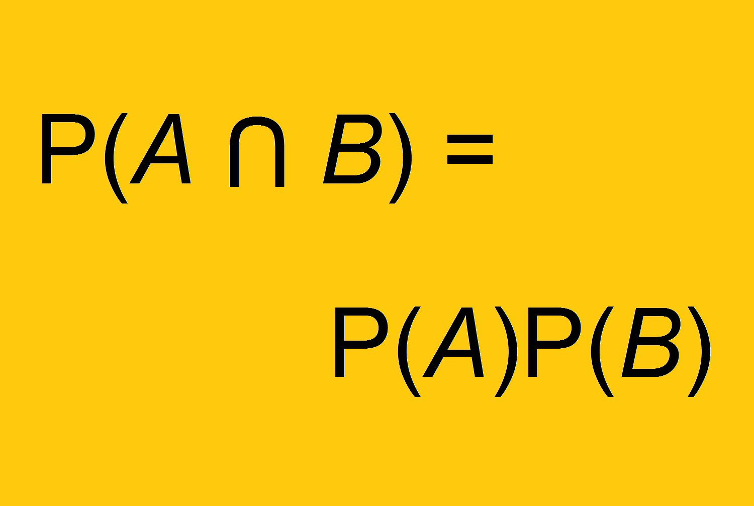
multiplication law for independent events

probability distribution

list of outcomes and their associated probabilities

discrete propability function

• probability that x can take a SPECIFIC value, a, is p(a): P[X=a] = p(a)

• p(x) is non-negative for all real x

• sum of p_j = 1 where j is all possible values that x can have

• 0 <= p(x) <= 1

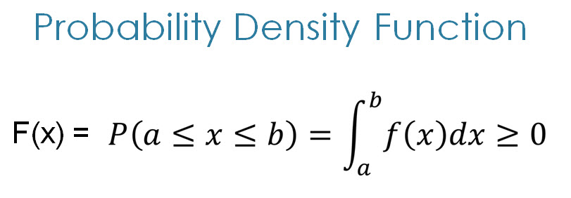
continuois propability distribution

• when a variable is continous, its probability distribution will be a smooth continuous curve

• probabilities are measures over an interval of values, not single point (ex. p(-1<x<1) instead of p(x=1))

continuous probability function

• f(x) is non-negative for all real x

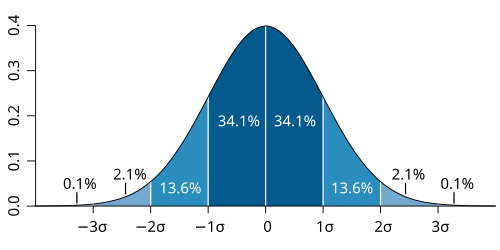
normal distribution

• N(u, o²)

• mean = median = mode

• 68% of data = mean +- 1SD

• 95% of data = mean +- 2SD

• 99.7% of data = mean +- 3SD

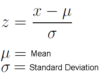
z-score

• how likely it is to get an observed value given that the data follows a normal distribution

• useful bc it converts any normal dist. into the standard normal N(0,1), making values across different distributions directly comparable

sampling distribution

probability distribution of a statistic drawn from repeated sampling

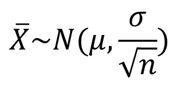
sampling distribution of sample mean

• mean of distribution = population mean

• SD of distribution (standard error) is population SD/sqrt of n (sample size)

• normal dist

• variance of distribution = (popuilation SF)² / n

• but we don’t know the population SD, so we estimate it using s (sample SD)

central limit theorem

for random sampling w n >= 30, the sampling distribution of the sample mean is approximately normal, regardless of the population data’s distribution shape

• useful bc we can still use characteristics of normal distribution for the mean’s distribution to build confidence intervals and perform significance tests even when population distribution is skewed.