MLE FINAL

:(

supervised learning

learning from labeled data (each example or instance in the dataset has a corresponding label)

• classification vs regression

unsupervised learning - def

learning from unlabeled data (must discover patterns in the data)

• clustering (K-means)

• dimensionality reduction

problems/tasks:

• density estimation

• outlier detection

• clustering

• dimensionality reduction (& visualization)

• association rule mining

semi-supervised learning

learning from partially labeled data

reinforcement learning

there is an agent that can interact with its environment and perform actions and get rewards

• learning policy (strategy for which actions to take) to get the most rewards over time

transfer learning

learning to repurpose an existing model for a new task

density estimation

model the (unknown) probability distribution function (pdf) from which data is drawn

outlier detection

identify data points that do not belong in the training data

clustering

goal: group similar data points together in “clusters”

• dataset: matrix X (n x m) — no labels

• clustering algorithms:

  • k-means clustering

  • DBSCAN

  • hierarchical clustering

• Need a holdout set — the clustering could overfir

  • Should train-test split or train-test-val split

dimensionality reduction (& visualization)

transform dataset into a low(er)-dimensional representation in a way that preserves useful information

association rule mining

discover interesting relationships between variables in the data

k-means clustering

• greedy iterative algorithm to assign points to clusters

• input: dataset X, integer k (hyperparameter — number of clusters)

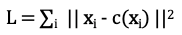
k-means — objective function

c(x_j) is the centroid of the cluster that x_j is assigned to

k-means algorithm

Initialization: random centroid for each cluster

Do until no change in clustering:

• assignment: assign each data point to the cluster with the closest centroid

• update: recalculate centroids from points assigned to each cluster

k-means — determine k

• guess or try different options

• Heuristics: silhoutte method or elbow method

• tune is as you would any other hyperparameter (if you have an objective metric to evaluate the quality of a clustering)

dataset has millions of features

training would be slow and model performance could suffer

curse of dimensionality

as dimensions increase, data becomes more sparse, making it harder to find meaningful patterns and causing distance-based algorithms to struggle.

• as the number of features increases, the amount of data required to generalize accurately grows exponentially, making data points appear as isolated islands

dimensionality of data is artificial

can reduce dimension without losing information

dimensionality reduction techniques

• projections (PCA)

• manifold learning (LLE, Isomap)

principal component analysis (PCA)

• method for linear transformation onto a new system of coordinates

  • the transformation is such that the principal components (coordinate vectors) capture the greatest amount of variance given the previous components

• linear decomposition/transformation

PCA — algorithm

• given data matrix X (n x m)

  • Mean-center it: subtract the mean of each feature

• compute covariance matrix X^TX (m x m)

• eigendecomposition gives principal components

  • use Single Value Decomposition (SVD)

  • Matrix W of eigenvectors is the transformation matrix (i^th column is the i^th principal component)

  • Eigenvalue λ_i gives the variance of the i^th principal component

PCA note

can to PCA on the correlation matrix instead of covariance matrix

PCA — inverse transformation

transform data back to the original space

• X’ = Z_k W_k^T

  • W_k^T is a k x m matrix

  • X’ is a (n x m) matrix

PCA — transformed data

Z_k = X W_k

• W_k is the transformation matrix with only the first k columns (m x k)

PCA — reduce dimensionality

to reduce dimensionality, can only keep the first k principal components

PCA - variance explained

(λ₁₊λ₂+...+λ_k) / ∑_i λ_i

Kernel PCA

• for non-linear dimensionality reduction

• use kernel trick (same un used for SVM)

Manifold Learning

Find mapping of dataset X into dataset Z embedded in R^p (Z_i ∈ R^p) for some integer p > m

• Such that (informally) Z preserves the local geometry of X

  • For example, if x_i and x_j are close (according to some distance metric), then z_i and z_j are also close

  • Want to preserve neighborhood structure

multidimensional scaling (MDS)

• compute euclidean distance d_ij between any two points x_i and x_j

manifold learning — algorithms

different algorithms aim to preserve different “local” properties

• multidimensional scaling (MDS)

• locally linear embedding (LLE)

• Isomap

• t-distributed stochastic neighbor embedding (t-SNE)

locally linear embedding (LLE)

express each data point as a linear combination of its closest neighbors

multidimensional scaling

preserve distances between points

isomap

• form a graph where points are connected to their closest neighbors

  • aims to preserve geodestic distance (i.e., shortest path distance)

t-distributed stochastic neightbor embedding (t-SNE)

• tries to keep similar data points close together, dissimilar data points far part

• mostly used for visualization

model formula

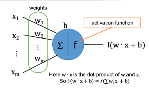
h_w,b(x) = f (w ^. x + b)

single nueron/unit

NN — types of layers

• dense (fully connected)

• convolutional

• recurrent

NN - activation functions

• identity / linear

• sigmoid

• tanH

• ReLU

• Softmax

NN — identity activation function

f(z) = z

• or none

NN — sigmoid activation function

f(z) = 1/(1 + e^-z)

NN — TanH activation function

f(z) = (e^z - e^-z) / (e^z + e^-z)

NN — ReLU activation function

f(z) = max(0, z)

NN — Softmax activation function

f(z_j) = exp(z_j / T) / ∑_i exp(z_i / T )

• note: in this case, the activation function is over an entire layer, not a single unit

NN — Loss

Make sure the loss function and activation function of the output layer are consistent with each other

Single Nueron — Linear Regression

one layer NN with a single neuron:

• Activation function: Linear

• Loss function: MSE

single neruon (binary) logistic regression

one layer NN with a single neuron

• Activation function: sigmoid

• Loss function: binary cross-entropy

Multi-Layer Perceptron (MLP)

• input layer (passthrough)

• one or more hidden layers

• output layer

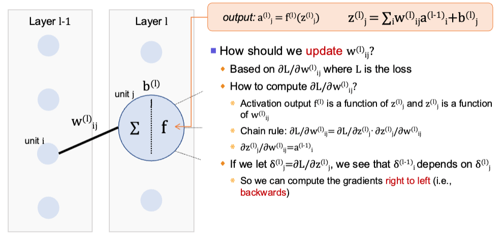
backpropagation — overview

reverse pass to measure error and propagate error gradient backwards in the network

• adjust the weights (parameters) to decrese the loss

backpropagation

how to compute gradients efficiently

gradient descent

how to update the parameters to minimize the loss given the function

backprop algorithm

• compute the forward pass for the mini-batch B saving the intermediate results at each layer

• compute the loss on the mini-batch b (compares output of network to labels/targets —> error)

• backwards pass: computes the per-weight gradients (error contribution) layer by layer

  • done using chain rule

• Stochastic gradient descent: update the weights based on the gradients

chain rule

if z depends on y and y depends on x:

dz/dx = dz/dy · dy/dx

backprop — illustration

Use NN

• complex learning task or complex data

• for many problems, NN provide the best performance

  • image classification/captioning tasks

  • speech recognition

  • natural language modeling

dont use NN

• can solve problem with simple model

• don’t have a lot of data

  • NN require a lot of data to achieve good performance

• need an explainable/interpretable model

  • there are some techniques to explain decisions from NN

universal approximation theorems

(feed-forward) NN can approximately represent any function

arbitrary width; bounded depth

true even if we have a single hidden layer as long as it can have arbitrarily many units

bounded width; arbitrary depth

true even if we have layers of bounded width, as long as the network can have arbitrarily many layers

NN architecture disadvantage

inconsistent activation function of output layer with the loss function

multiclass classification with cross-entropy loss, softmax activation for output layers

okay

regression with MSE as loss, tanh activation for output layer

Fail

regression with MSE as loss, linear activation for output layer

okay

funnel trick

for supervised learning, we typically have large input feature vectors and small output vectors

• should make the network look like a funnel

multiclass classification with 10 classes and m = 100 input features

(input, hidden layer 1, hidden layer 2, hidden layer 3, output layer)

• 100, 64, 32, 16, 10

Activations:

• output: softmax

• elsewhere: ReLU

deep NN

anything NN with two or more hidden layers

Deep NN (DNN) challenges

endless options for netwrok architecture/topology

• # of layers, units per layer, connections between units, activation functions, weight intialization method

DNN - hyperparameters related to learning

• optimizer

• learning rate

• decay/momentum

• (mini) batch size

• # of epochs

DNN - Number of Hidden layers

Deep > shallow: for the same number of parameters, more hidden layers is better than wider layers

• parameter efficiency

number of units in each layer - funnel approach

make the network look like a funnel

number of units in each layer - “stretch pants”

make hidden layers wider than what you need and then regularize (ex. dropout)

DNN - activation function

hidden layers — ReLU or ReLU variants

• faster to compute than alternatives

• GD less likely to get stuck

output layer

• multiclass classification: softmax

• binary classification or multilabel: sigmoid

• regression: linear (no activation function)

DNN learning rate

start with low value (0.00001) then multiply by 10 each time and train for a few epocs

• once training diverges — have gone too far

training diverges

the model isn’t settling toward a stable solution — it’s going in the wrong direction instead of improving

• loss error start to increase instead of decreasing

DNN - optimizer

use ADAM or SGD

DNN — batch size

• small batch approach: ex. 32, 64, 100

• large batch approach: the largest size that fits your GPU’s RAM and use learning rate warmup

DNN — number of epochs/iterations

use early stopping

• stop training before the model starts getting worse on new (unseen) data

• stop at the point where validation performance is best, not where training loss is lowest

vanishing gradient

gradient vector becomes very small during backprop

• difficult to update weights of lower/earlier layers — training does not converge

exploding gradient

gradient vector becomes very large during backprop

• difficult to update weights of lower/earlier layers — training does not converge

training converges

with GD, the process has found (or gotten very close) to a minimum of the loss function — each additional step makes little to no difference

unstable gradients

layers of a dnn learn at very different rates

exploding/vanishing gradient mitigations

• weight initialization method

• non-saturating activation functions

• batch normalization

• gradient clipping (for exploding gradient)

• skip-connections (CNNs)

glarot intialization (Xavier intialization)

• Let n_in: number of inputs, n_out: number of outputs n_avg = (n_in + n_out)/2

• Gaussian (for sigmoid activation): mean 0, variance σ2 = 1/n_avg

• Uniform (for sigmoid activation): in [-r, r] where r = [3/n_avg]^1/2

note: biases are initialized to 0

He intialization

Gaussian (for ReLU): mean 0, variance σ² = 2/n_avg

• note: biases are initialized to 0

non-saturating activation functions

ReLU + ReLU variants

dying ReLUs

• a neuron can die when the weighted sums of its input are negative (for all examples in the training data)

ReLU variants

• Leaky ReLU

• ELU

• SELU (Scaled ReLU)

these will not let neurons die because they can output negative values

Leaky ReLU

LeakyReLU_a(z) = max{az, z}

e.g.: a = 0.01

ELU

ELU_a(z) = z if z ≥ 0 and a (e^z - 1) otherwise (z < 0)

e.g., a = 1

activation functions — rating

ELU > leaky ReLU > ReLU > Tanh > Sigmoid

use ReLU in most cases, ELU if there is extra time because network will be slower

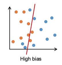
bias

error due to incorrect assumptions in the model

• inability to capture the true relationship

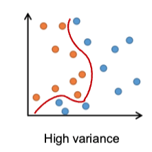
variance

sensitivity to small variations in the training data

strategies to lower bias

• increase model complexity

• use more features

strategies to lower variance

• reduce model complexity

• use more training data

DNN reg technique — early stopping

stop once the validation loss is at its minimum (before it starts to go back up)

DNN reg technique — L₁ or L₂ reg

• L₁: penalty term λ∑_i |w_i|

• L₂: penalty term λ∑_i |w_i|²

DNN reg technique — max-norm reg

the norm of weights incoming to each neuron is at most r (hyperparameter): ||w||₂ < r

note: this is not added to the loss — after each training step, the weights are scaled to ensure ||w||₂ < r

DNN reg technique — drop out

idea: during training, each neuron has a probability p of being dropped out (it will be ignored for this step)

• hyperparameter p is called the dropout rate

• after training: we do not drop any neurons anymore (but need to adjust connection weights)

generalization error

aka out-of-sample error or risk

• prediction error on unseen data

• related to overfitting: if the model overfits, then the generalization error will be large

bias² + variance + irreducible error

bias-variance tradeoff

• increasing model complexity — lower bias

• decreasing model complexity — lower variance

double descent

• unexpected and sudden change in test error as a function of model complexity (# of parameters)

  • Note: not all settings/models/data yield exactly two descents (e.g., sometimes there are three or more)

grokking

NN learns to generalize suddenly well after the network has overfitted

note: this occurs in very specific settings (specific tasks, small “algorithmic datasets”, complex neural networks)