CFA - Quant 1

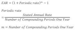
Effective Annual Rate (EAR)

*Rate and Returns

Rate of interest that an investor can earn (or pay) in a year after taking into consideration compounding

Nominal Risk-Free Rate

*Rate and Returns

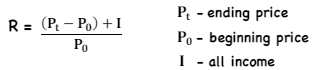
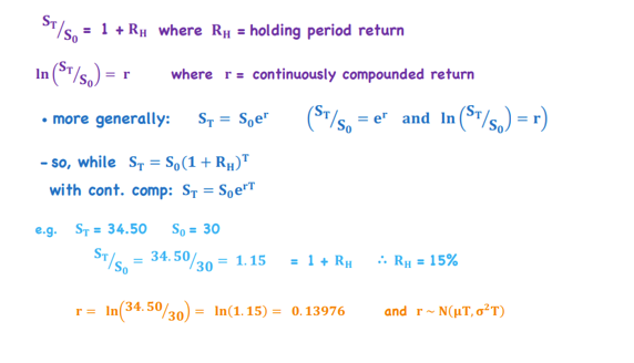
Holding Period Return (HPR)

*Rate and Returns

Return on an asset/portfolio over the period during which it was held

Multi-Period HPR

*Rate and Returns

Arithmetic Mean

*Rate and Returns

• When it's used: Used to estimate E(R) over one period

Geometric Mean

*Rate and Returns

• When it's used: Used to estimate average E(R) per period over multiple periods, use for returns

• R_G <= R_A

• FV = PV(1 + R_G) - measures an investment’s terminal value over multiple periods

Harmonic Mean

*Rate and Returns

• Reduces the effect of outliers & underweight their impact

• When it’s used: Multiples/ratios, dollar-cost averaging, average price per unit

• Relationship w other means: R_A (overweight) x X-bar_H (underweight) ~ R_G²

Trimmed Mean & Winsorized Mean

*Rate and Returns

Trimmed: Remove a percentage from both largest and smallest, e.g. 8% trimmed - 16% total (common with CPI)

Winsorized: Replacing values at both ends with cutoff value

Money-Weighted Return (IRR, YTM)

*Rate and Returns

• Discounting CFs

• What your money earned, not the typical $1

• More sensitive to the timing and amount of withdrawals/additions to the portfolio (e.g. if you committed more money to a poor performance year, your mwrr < R_A)

Time-Weighted Return

*Rate and Returns

= R_G (same as geometric mean)

Represents growth of $1 over a given period

Method

• Break investment period into holding periods

• Calculate each HPR, compound HPRs, express annually

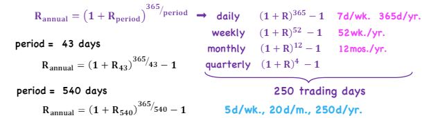
Annualized Return

*Rate and Returns

• All rates/returns are quoted annually

• Can be misleading - assumes that returns can be repeated

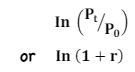
Continuously-Compounded Return

*Rate and Returns

• Continuously compounded return is equivalent to its annual counterpart

• To get back to annual rate: e^rc - 1

Gross v. Net Return

*Rate and Returns

Gross: What the fund earns - return before deductions for management. exp, custodial fees, taxes… BUT after trading expenses

Net: What the investor earns

Real Return

*Rate and Returns

After-tax real return - Investor measure of growth in purchasing power of portfolio

Leveraged Return

*Rate and Returns

Use leverage when return on portfolio R_p > cost of debt r_d (if you’d earn more an more in an investment than you would from borrowing money)

R_L = R_P/P_E = [R_P x (Total Value) - (Debt Value x r_b)]/Equity Value

R_L = R_P + V_B/V_E*(R_p - r_d)

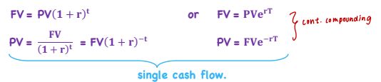
Zero-Coupon Bond/ZCB (Single CF)

*TVM - Fixed Income

Sold at a discount, matures at par

Ex. T-bills

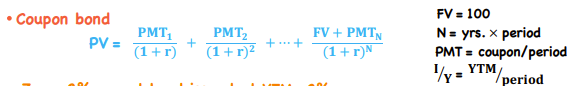
Coupon Bond

*TVM - Fixed Income

Investor receives a number of interest payments over time and par at maturity

Ex. Notes, bonds

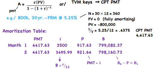
Fully Amortizing Bonds

*TVM - Fixed Income

Investor receives level payments of both interest and principal

Ex. Mortgage, auto loan

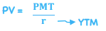
Perpetuity

*TVM - Fixed Income

Ex. bonds, preferred shares

Annuity

*TVM - Fixed Income

Ex. mortgage, car loans

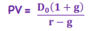
Perpetuity (Constant Dividend)

*TVM - Equity

Ex. Many REITs

Growing Perpetuity (Constant Growth Dividend)

*TVM - Equity

Ex. Commercial real estate - to calculate property value

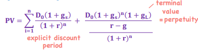
2-Stage Model (Growth Moving to Value)

*TVM - Equity

Rate of growth will slow down in the long-term

• Explicit discount period - Similar to coupon bonds

• Terminal value - Perpetuity (discount terminal value to this PV)

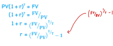
Implied Return on Fixed Income

*TVM - Fixed Income

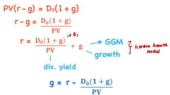
Required Return and Implied Growth of Equity

*TVM - Equity

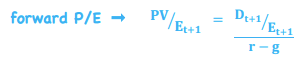
Forward PE

*TVM

• PE formula: Constant growth dividend formula / Equity

• Numerator becomes dividend payout ratio (DPR), D₀ / E

• Forward dividend payout ratio = DPR * (1 + g)

• If forward dividend OR growth rate (g) is expected to increase, the stock/index will trade a higher forward multiple

• Higher required return (r) leads to lower multiple (greater denominator)

Principle of No Arbitrage

*TVM

Cash flow additivity - 2 economically equivalent strategies should have the same price

Calculate PV of two CFs, select the higher one OR take the difference in CFs (A-B), if PV>0, choose A, else B

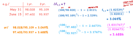
Implied Forward Rate

*TVM

f_{when, what} — f_3,4 = forward rate that begins in 3 years and lasts 4 years

Can also just divide the two PV’s to get implied forward rate

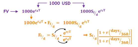
Forex - Foreign Exchange Rate

*TVM

F_f/d = Forwards/futures price

S_f/d = Spot rate (foreign/domestic)

r_d = Domestic rate

r_f = Foreign rate

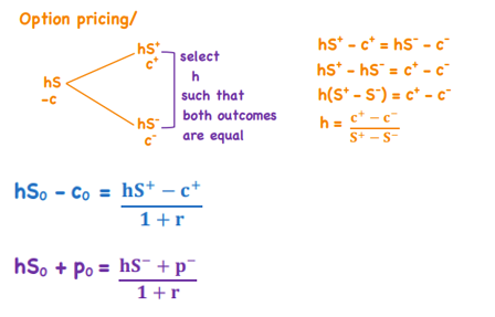
Option pricing

*TVM

h = Hedge ratio

• Short a call (-)

• Long a put (+)

Notations for X and Y Terms

X-bar/Y-bar = Sample mean

X-hat/Y-hat = Estimate

X_i/Y_i = Specific values of X/Y

Dispersion

*Statistical Measures of Asset Returns

• Variability around the central tendency

• A measure of risk or uncertainty

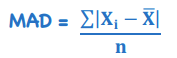
Mean (of the) Absolute Deviation

*Statistical Measures of Asset Returns - Dispersion

Average distance between each data point and the mean

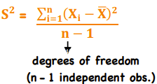
Sample Variance

*Statistical Measures of Asset Returns - Dispersion

Average/expected deviation from the mean

Square root of sample variance = sample SD

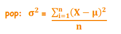
Population Variance

*Statistical Measures of Asset Returns - Dispersion

Square root of population variance population SD

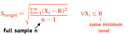
Downside Deviation (ex. Target Semideviation)

*Statistical Measures of Asset Returns - Dispersion

• A measure of the risk of being below a certain target B

• As B increases, S_target also increases

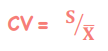
Coefficient of Variation (CV)

*Statistical Measures of Asset Returns - Dispersion

• Measure of relative dispersion

• For returns, CV measures the risk per unit of return

• Lower = better, since it indicates less uncertainty, tighter distribution

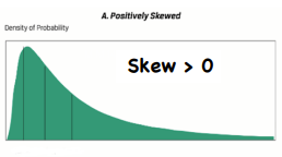
Positive Skew

*Statistical Measures of Asset Returns - Distribution

• Mean > median > mode (highest point of distribution)

• Ex. Long options portfolio - a lot of small losses & a few large gains

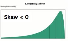
Negative Skew

*Statistical Measures of Asset Returns - Distribution

• Mean < median < mode (highest point of distribution)

• Ex. Short options portfolio - a lot of small gains & a few big losses

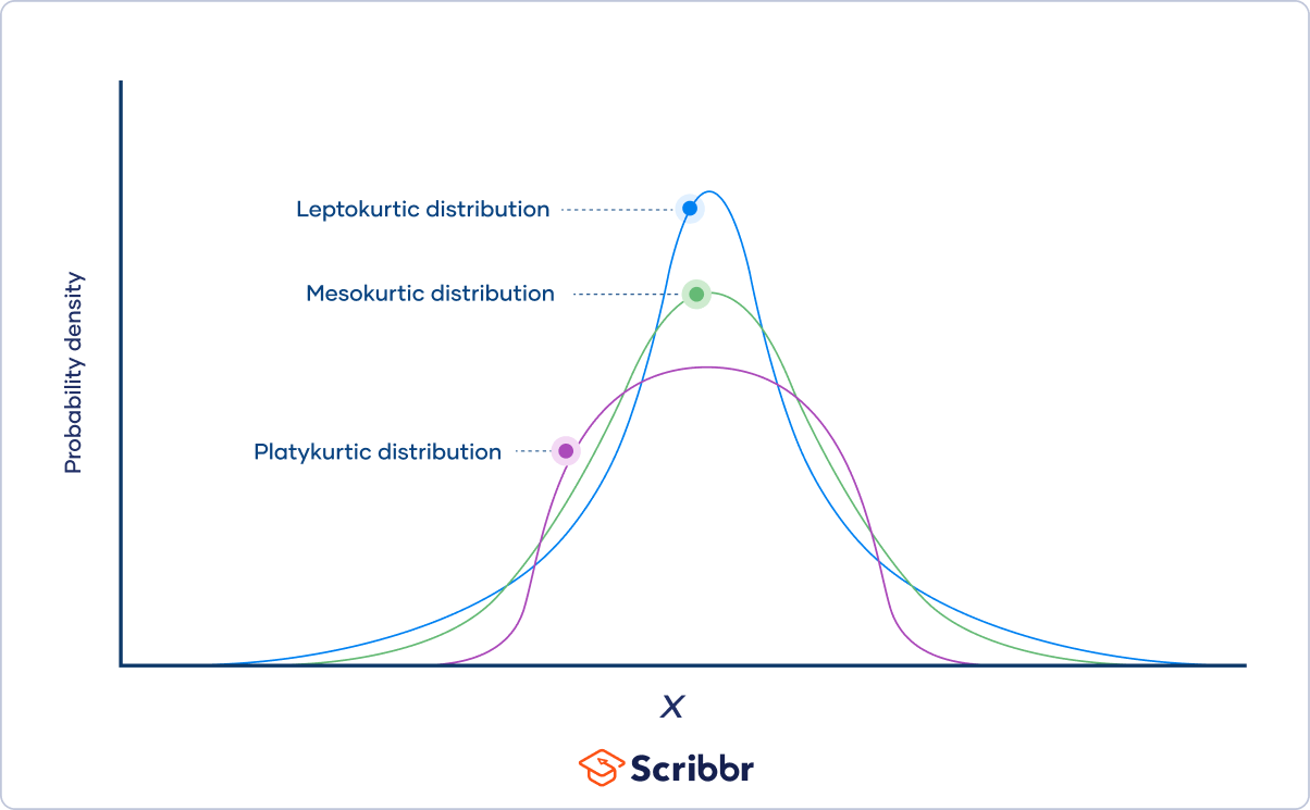
Kurtosis

*Statistical Measures of Asset Returns - Distribution

Measures how much of a probability distribution falls in the tails instead of its center (Normal distribution has K = 3)

Types:

• Leptokurtic (K > 3, K_e > 0) - More observations around the mean with more weight in the tails

• Mesokurtic (K = 3, K_e = 0)

• Platykurtic (K < 3, K_e < 0) - Few observations around the mean with less weight in the tails

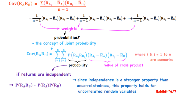
Covariance

*Statistical Measures of Asset Returns - Correlation

• Joint variability of two random variables

• S_XY > 0 when the variables covary together (observation of X above its mean & observation of Y above its mean, vice versa with observations below means)

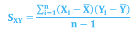
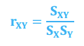
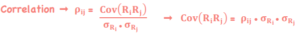
Correlation

*Statistical Measures of Asset Returns - Correlation

Measures linear association between two variables

• Maximum diversification - No linear relationship (r = 0)

• Perfect replication - Perfect positive correlation (r = 1)

• Perfect hedge - Perfect negative correlation (r = -1)

Limitation: Spurious correlation - chance relationship with a third variable a (X/a, Y/a, still correlation r_XY)

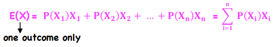
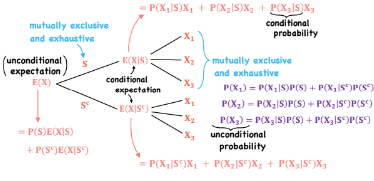
E(X) - Expected Value of a Random Variable

*Probability Trees and Conditional Expectations

Probability-weighted average of the possible outcomes - estimation of the ‘true’ population mean based on a sample

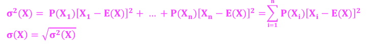
Variance/SD of a Random Variable (σ²/σ)

*Probability Trees and Conditional Expectations

Probability Tree

*Probability Trees and Conditional Expectations

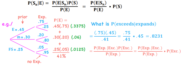
Bayes’ Formula

*Probability Trees and Conditional Expectations

Definition - A method for updating prior probabilities based on new information (switching conditionals)

Method:

• 1) Find total probability of the condition

• 2) Find each sub component that makes up the condition

• 3) Divide sub-component by total to update all prior probabilities

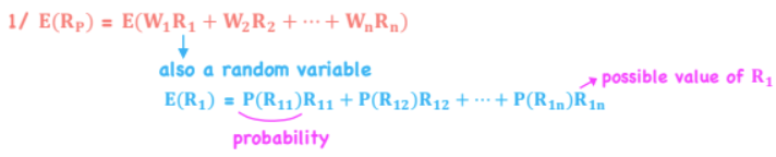
E(R_p) - Expected Value of Return

*Portfolio Mathematics

Portfolio Return - measure of expected reward

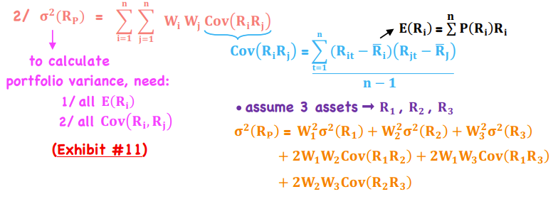
Portfolio Variance

*Portfolio Mathematics

Covariance of portfolio with 2 asset classes i and j = w_i²(R_i) x w_j²(R_j)× 2w_iw_jCov(R_iR_j)

For n securities/asset classes, there are:

• n variances (ex. n = 5)

• n² - n covariances (ex. 25 - 5 = 20 cov)

• (n²- n)/2 distinct covariances (ex. 20/2 = 10 unique cov)

Portfolio risk is lowered by selecting assets with 0 or negative covariance

Correlation

*Portfolio Mathematics

Covariance as a Joint Probability Function for Returns

*Portfolio Mathematics

Moving away from having expected return of an asset class to having expected returns based on possible scenarios (need joint probability)

Product of Deviations x Probability of Condition

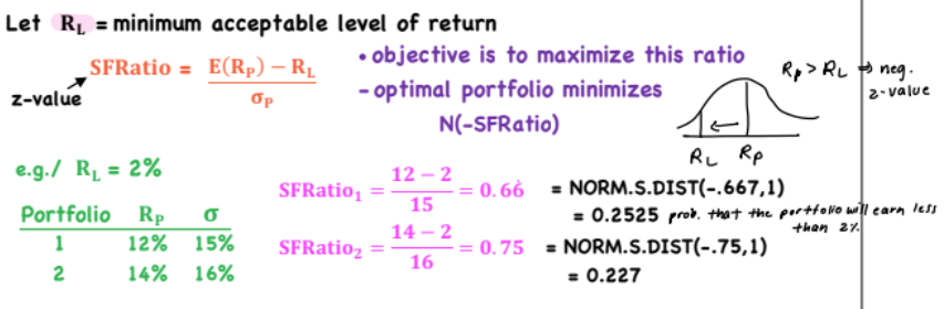
Shortfall Risk

*Portfolio Mathematics

• Definition: The risk a portfolio value (or return) will fall below some minimum acceptable level over some time horizon

• Objective is to maximize this ratio - Optimal portfolio minimizes N(-SFRatio)

• NORM.S.DIST(-SFRatio, df) - Result is the probability that the portfolio will earn less than R_L

• If R_L = R_f then SFRatio = Sharpe Ratio

Lognormal Distribution

*Probability Distributions

Used to model the probability distribution of asset prices - described by the mean and variance of its associated normal distribution

Relationship between lognormal and normal distribution - A variable Y follows a lognormal distribution if LN(Y) is normally distributed

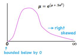
Lognormal Distributions - Return

*Probability Distributions

Used to model asset prices when using continuously compounded asset returns - cannot be negative (bounded below by 0)

Lognormal Distribution - Volatility

*Probability Distributions

Annualized SD of the continuously compounded daily returns of the underlying asset

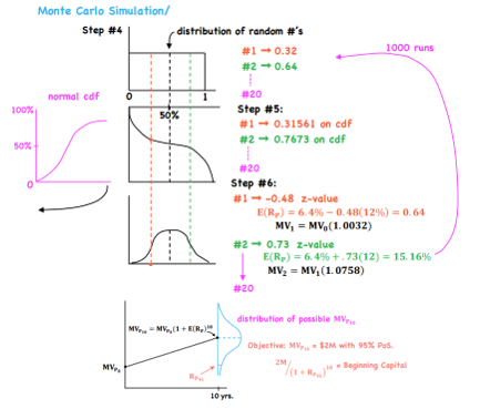
Monte Carlo Simulation

*Probability Distributions

Situation: We have a number of variables & we know how they behave since some common probability distributions describe the behavior of these variables - What are some other possible pathways of meeting my goals in the future with my portfolio return and SD?

Method:

• 1) Specify quantity of interest (ex. MV_p in 10 years)

• 2) Specify a time grid - K sub-periods with time increment over the full time horizon (time increment = 6 months, 20 sub-periods)

• 3) Specify distributional assumptions for the key risk factors - E(R_p) & σ

• 4) Draw standard normal random numbers for each key risk factor over each K sub-periods (random number generator produces a distribution of random numbers from 0 to 1, all equally likely)

• 5) Map area under cdf (flip it?)

• 6) Obtain z-values to map out (approx. 1,000 runs)

• 7) Simulation will produce a distribution of outcomes around the point estimate of expected return at a certain time

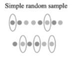
Simple Random Sampling

*Estimation - Probability Sampling

• Definition: A subset of a larger population such that each element has an equal probability of being selected

• Sample size = n, 1/n probability of being selected

• Useful when data are homogenous

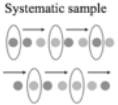
Systematic Sampling

*Estimation - Probability Sampling

• Definition: Select every K^th element until the desire sample size is reached

• No logical ordering/selection process, used when the population is too large to code

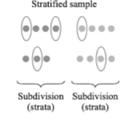
Stratified Random Sampling

*Estimation - Probability Sampling

• Definition: Population is sub-divided into sub-populations based on one or more classifications. Simple random samples are drawn from each sub-population, which is pooled to form main sample

• Each sub-sample is proportionate to the size of it’s sub-population, guaranteeing representation & more precision

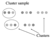
Cluster Sampling

*Estimation - Probability Sampling

• One-stage cluster sampling: Population is divided into clusters, and some of these clusters are randomly selected into your sample

• Two-stage cluster sampling: Sub-samples are selected from each cluster

• Cost & time efficient, but usually results in lowest precision

Sampling Error

*Estimation and Sampling

• Definition: Difference between observed values of a statistic and population parameters as a result of using just a subset of the population. Deviations of sample drawn from true population

• Tapers at around n=200

Non-Probability Sampling

*Estimation and Sampling

Types:

• Convenience sampling - Observations are selected that are easy to obtain or accessible (ex. prof uses students)

• Judgemental sampling - Select observations based on experience and knowledge (ex. auditor selectively reviewing accounts)

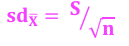
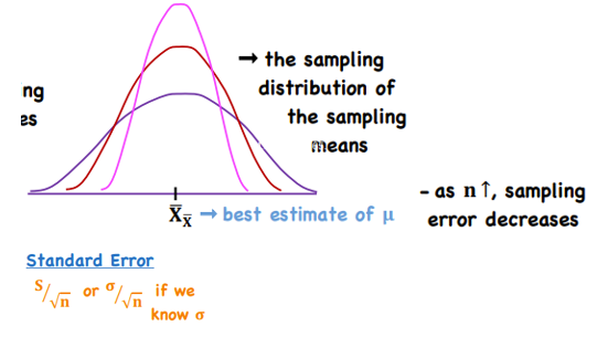
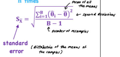
Standard Error

*Estimation and Sampling

• Definition - Standard deviation of sample means around population means

• Central Limit Theorem - Sampling distribution of the mean will always be normally distributed, as long as the sample size is large enough (tapers at around n=200)

z-values

60% = 1

90% = 1.64

95% = 1.96

99% = 2.58

Bootstrap Method

*Estimation - Resampling

• Method - Draw 1 observation, record & replace n times to create a distribution (rather than estimating)

• Uses computer simulation

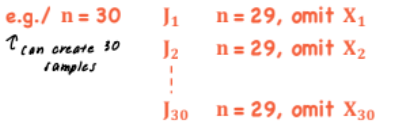
Jackknife Method

*Estimation - Resampling

• Method - Omit one observation from a sample, one at a time

• Will produce similar results from sample to sample

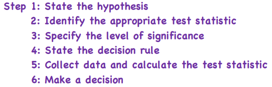
Hypothesis Testing

Test to see whether a sample statistic is likely to come from a population with the hypothesized value of the population parameter - Does X-bar = μ₀?

*Typically want to reject null, and accept alternative

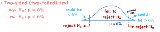
Two-sided (Two-Tailed) Test

*Hypothesis Testing

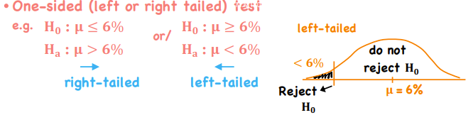
One-sided (Left-Tailed or Right-Tailed test) Test

*Hypothesis Testing

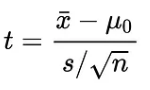
Test of a Single Mean

*Hypothesis Testing - t-Distributed Test Statistic

df = n - 1

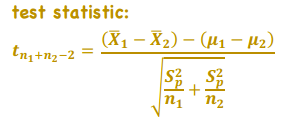
Test of the Difference in Means

*Hypothesis Testing - t-Distributed Test Statistic

Are X-bar₁ and X-bar₂ from the same population or different populations?

df = n₁ + n₂ - 2

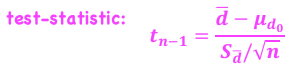
Test of the Mean of Differences (Paired-Sample t-Test)

*Hypothesis Testing - t-Distributed Test Statistic

Is the mean difference between two sets of observations 0?

df = n - 1

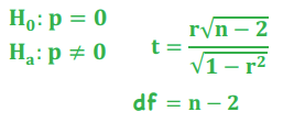
Test of a Correlation

*Hypothesis Testing - t-Distributed Test Statistic

*Parametric Test of Correlation

Is there a statistically significant correlation between two variables?

df = n - 2

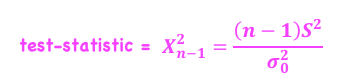
Test of a Single Variance

*Hypothesis Testing - Chi-square-Distributed Test Statistic

Is the variance of the population equal to a specific value?

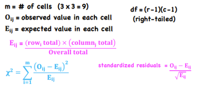
Test of Independence

*Hypothesis Testing - Chi-square-Distributed Test Statistic

*Non-Parametric Test of Independence

Categorical Data - Values that describe a quality or characteristic (nominal, ordinal)

Are these classification types independent? ex. Are growth stocks likely to be any size or are they more likely to be large-cap stocks?

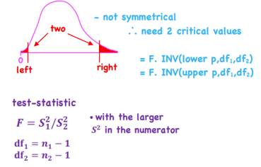
Test of the Difference in Variances

*Hypothesis Testing - F-Distributed Test Statistic

Are the variances of two populations equal? ex. Comparing the volatility of two funds

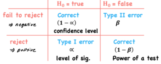
Level of Significance

*Hypothesis Testing

• Alpha & beta have an inverse relationship - Only way to decrease both is by increasing n

• Type I error: False positive

• Type II error: False negative

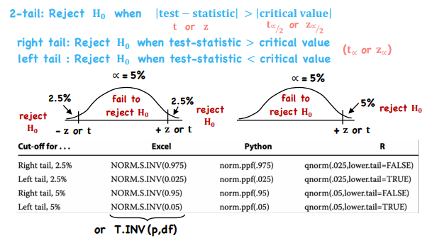
Decision Rules + Excel Formulas

*Hypothesis Testing

• NORM.S.INV( ) - probability in, critical value out

• NORM.S.DIST( ) - critical value in, probability out

OR

• T.INV (p, df) - probability in, critical value out

• T.DIST (val, df) - critical value in, probability out

Non-Parametric Testing

• When data do not meet distributional assumptions (n <30), population is non-normal)

• When there are outliers (test of median vs mean)

• When data are given in ranks or use ordinal scale (NO IR)

• Hypothesis doesn’t concern a parameter (ex. Is a sample random?)

Spearman Rank Correlation Coefficient (r_s)

*Non-Parametric Test of Correlation

Definition - Essentially a correlation calculated on rank values, not on the actual values of the observation

Method:

• 1) Rank all X from largest to smallest (1 - n). If there’s a tie, put in an average rank

• 2) On original data set, calculate d_i² = (rank X_i - rank Y_i)²

• 3) Calculate r_s

• 4) If n > 30, test r_s

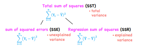
Total Sum of Squares (SST)

*Linear Regression

The sum of all squared differences between the mean of a sample and the individual values in that sample

Sum of the Squares Error (SSE) or Residual Sum of Squares (RSS)

*Linear Regression

The sum of difference between observed and predicted values

Goal of regression is to compute a line of best fit that minimizes the sum of the square deviations between observed and predicted values of Y

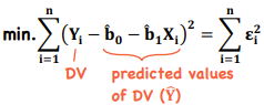
Linear Regression (components)

Linear Regression Assumptions

*Linear Regression

1) Linearity - The relationship between X&Y is linear in the parameters b₀ and b₁ (IV is not random)

2) Homoscedasticity - Variance of the dependent variable is the same for all observations

3) Independence - The pairs (X,Y) are independent of each other; error term is uncorrelated across observations (no serial correlation - ability to predict likelihood of next error being +/-)

4) Normality - Error term is normally distributed

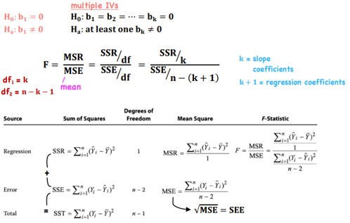
Total Sum of Squares (SST)

*Linear Regression - Analysis of Variance

SST (total SS) = SSE (unexplained SS)+ SSR (explained SS)

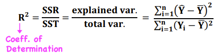
Coefficient of Determination

*Linear Regression - Analysis of Variance

Measures the fraction of the total variation in the DV that is explained by the IV (goodness of fit measure)

NOT a statistical test

Statistical Test - ANOVA test

*Linear Regression - Analysis of Variance

• F-Stat Excel Function - F.INV(prob, SSR df, SSE df)

• Standard Error of the Estimate/Regression (SEE) = (MSE)^1/2 - The smaller the SEE, the more accurate the regression

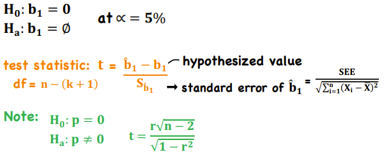
Hypothesis Tests of b-hat₁

*Linear Regression - Hypothesis Test

• Test - Is it significantly different from 0?

• t-stat Excel Function - T.INV (prob, n-k-1)

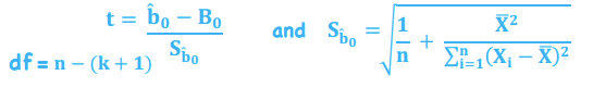
Hypothesis Tests of b-hat₀

*Linear Regression - Hypothesis Test

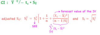
Prediction Interval for Y-hat

*Linear Regression

2 sources of error that we need to account for in the :

• Y residuals

• b-hat₀ and b-hat₁ are estimated with error

Properties

• 1) The better the fit of the regression model. the lower S_e², the lower S_f² (SE of forecast)

• 2) Larger n = smaller S_f²

• 3) The closer X_f is to X-bar = smaller S_f²

Log-Lin Model

*Linear Regression - Functional forms of the regression model

Relative change in Y for absolute change in X

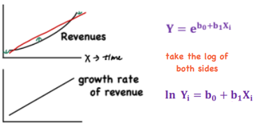
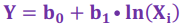
Lin-Log Model

*Linear Regression - Functional forms of the regression model

Absolute change in Y for the relative change in X

Ex. Y = Percent, X = $B in Revenue

Log-Log Model

*Linear Regression - Functional forms of the regression model

Relative change in Y_i for a relative change in X_i