Eco 231 - Exam 2 Questions

Prediction Equation (3 independent variables)

y(hat) = b0 + b1X1 + b2X2 + b3X3

F-test for overall fit in multiple regression

• checks whether the model explains variation in the dependent variable

• F=MSE/MSR​

Implication of the F-test for a multiple regression

• Reject H₀:
  → Statistically significant
  → At least one predictor variable is useful in explaining Y

• Fail to reject H₀:
  →Not better prediction than the mean of Y alone

Null and alternate hypothesis for regression with 4 independent variables

Equation:

Y=b0​+b1​X1​+b2​X2​+b3​X3​+b4X4+ei

Null hypothesis (H₀):

H0 = β1=β2=β3=B4=0

→ None of the independent variables explain Y

Alternative hypothesis (H₁):

At least one βi≠0

→ At least one independent variable helps explain Y

F-stat formula explaination

• MSR (Mean Square Regression)
  Measures how much variation in the dependent variable is explained by the model.

• MSE (Mean Square Error)
  Measures the unexplained variation (the residual/error).

• If F is large → the model explains significantly more variation than noise → predictors are useful

• If F is close to 1 → model is not much better than random noise

• A large F-statistic (with a small p-value) leads you to reject H₀, meaning the model is statistically significant overall.

• Look at P-value

Polynomial Regression

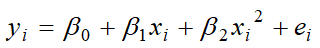
How do we interpret the coefficient on a quadratic variable in a regression?

1. Curve Direction

• b2>0 → upward (U)

• b2<0 → downward (n)

2. Marginal effect is not constant

3. Turning point

   1. If b2>0 → min

   2. If b2<0 → max

What is the logarithm transformation of the x and y variables?

The % change in y for every 1% change in x

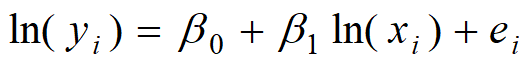
What does the coefficient on the x variable tell us after a log-log transformation of both the x and y variables?

the elasticity

What is an indicator/dummy variable

• variable that replaces a qualitative value

• difference in the predicted outcome between the group coded as 1 and the group coded as 0

When there are m different groups in the data for an independent variable, how many dummy variables are needed to indicate the m groups?

one less than m

What does the coefficient on a dummy variable tell us in a regression model?

• The average difference in Y between the group with D=1 and the group with D=0

  • If β1>0 → the “1” group has a higher outcome than the baseline

  • If β1<0 → the “1” group has a lower outcome

  • If β1=0 → no difference between groups

Can you show the difference using graphs?

• Lower line = baseline group d=0

• Upper line = dummy variable d=1

• Vertical distance between lines =b1

What is an interaction term in a regression?

• The effect of one variable on the outcome depends on the level of another variable.

  • The impact of X, changes when Z changes

What does the coefficient on the interaction of a dummy variable and an independent variable (x) tell us?

Y=β0​+β1​X+β2​Z+β3​(X⋅Z)+ϵ

• X⋅Z is the interaction term

• β3​ tells you how the effect of X changes with Z

Can you show the difference using graphs?

• When Z=0:

  • Y=β0+β1X

• When Z=1:

  • Y=(β0+β2)+(β1+β3)X

• The intercept is different (shift up/down)

• The slope is also different (lines are not parallel)

  • The difference in slopes is caused by the interaction term β3

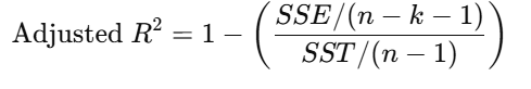
How is adjusted R-square different from R-square?

R-squared

• Measures the percentage of variation in Y explained by the model

• R2 always increases (or stays the same) when you add more variables

Adjusted R-Squared

• Used when you have to compare 2 regressions

• Adjusts R2 for the # of independent variables

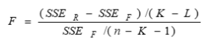
How to use adjusted R-square to compare reduced vs. full model in regression analysis?

• SSEr and SSEf are the error sum of squares for the reduced and full model

• K and L are the number of independent variables in the full and reduced models ​

What other criteria could you use for model selection?

• stepwise regression

  • begin with a simple regression then add more independent variables as controls

• backward elimination method

  • begin with full model (F) then eliminate insignificant independent variables in reduced model (R)

How to assess linear assumptions?

Points in a straight trend are linear

How to correct for violations of linearity assumption?

• Add a lagged value of the dependent variable as an explanatory variable

What are the ZINE assumptions for multiple regression models?

• Zero as the expected value for ei​

• Independence of errors​

  • Error values are statistically independent​

• Normality of errors​

  • Error values are normally distributed for any given set of X values​

• Equal Variance (also called Homoscedasticity)​

  • The probability distribution of the errors has constant variance​

How to assess the assumption of constant variance?

points in straight trend are constant

Heteroscedasticity

• variance of the error terms is not constant across observations

• fan shape” in residual plots

• makes standard errors wrong

  • messes up hypothesis tests and confidence intervals

How to correct heteroscedasticity?

• robust standard errors

• Transform dependent or independent variables

How to assess the assumption of normality for disturbance distribution?

• normal probability plot should be a straight line

• 68% of the standardized residuals should be between -1 and 1

• 95% should be between -2 and 2

• 99% should be between -3 and 3​

How to correct for violations of normality?

• If the sample size is greater than 30, normality assumption is not a concern​

• For small sample, use Box-Cox transformation toy: yp where 0<p<1​

How to assess the assumption that the disturbances are independent?

• Autocorrelation of residuals in time-series data​

Et = PEt-1 + Ut where 0 < p < 1​

• Test for first-order autocorrelation​

  • residual analysis

  • Durbin-Watson test ​ ​

Durbin Watson Test

• Residual analysis for time series data​

• The d statistic for Durbin-Watson test​

  • If residuals are uncorrelated, d = 2​

  • If residuals are positively correlated, d <2​

  • If residuals are negatively correlated, d> 2

How to correct violations of independence or autoregressive errors?

Add a lagged value of the dependent variable as an explanatory variable

What is correlation matrix?

are the pairwise correlations greater than 0.5?

How to deal with collinearity problem in regression?

• The presence of a high degree of multicolinearityamong explanatory variables can cause:​

  • insignificant coefficients on independent variables

  • unstable regression coefficients ​

• Detecting multicollinearity​

  • Correlation matrix: are pairwise correlations greater than 0.5?​

  • Large F statistic for regression but small t statistics (low p value) for estimated coefficient​

• Correction for multicollinearity​

  • Remove those variables that are highly correlated with others​

How to detect outliers?

use standardized deviation (ef), focusing on those with a value greater than 2​

How to correct outlier problem?

• Transformations:

  • log(X) or log(Y)

• Robust regression

What are the four components in a time series dataset?

• Trend component (T)

• Seasonal component (S) ​

• Cyclical component (C)​

• Irregular component (R)

How do you identify them?

Trend

• overall pattern

Seasonal

• part of the variation that fluctuates in a stable way over time

Cyclical

• regular cycles in the data with periods longer than one year

Irregular

• part of the data not explained by the model

Smoothing Method

• smooth away” the rapid fluctuations and capture the underlying behavior​

• recent behavior is a good indicator of behavior in the near future​

• Smoothing out fluctuations is generally accomplished by averaging adjacent values in the series

Simple Moving Average (SMA(4))

Yt = (Yt + Yt-1 + Yt-2 +Yt-3) / 4

Yt-1(hat) = Yt(hat)

Exponential Smoothing

EMA(0.7) = Yt(hat) = 0.7Yt + 0.3Yt-1(hat)

Y1(hat) = Y1

Autoregressive model

Yt(hat) = b0 + b1Yt-1 + b2Yt-2 + b3Yt-3

 How is autoregressive model different from smoothing method?

Autoregressive

• uses past values of the series itself

• depends on lagged values of Y

• statistical model to analyze structure

Smoothing

• uses past observations and forecasts

• depends on weighted averages of past values

• forecasting technique

Estimation equation for the autoregressive model with 3 lags

y(hat) = b0 + b1Ylag1 + b2Ylag2 + b3Ylag3

What is a multiple regression-based model for time series data with seasonal factors?

Yt​=β0​ + β1​t + β2​D1 ​+ β3​D2​ + ⋯ + βk​Dk​ + ϵt​

How do you represent the 4 quarters in a regression model?

Step 1: create dummy variables (3)

• D1​=1 if Q1, else 0

• D2=1D_2 = 1D2​=1 if Q2, else 0

• D3=1D_3 = 1D3​=1 if Q3, else 0

Step 2: Write regression model

Yt​=β0​+β1​D1​+β2​D2​+β3​D3​+ϵt​

Step 3: Interpret the coefficents

• β0​ → mean value in Q4 (baseline)

• β1\beta_1β1​ → difference between Q1 and Q4

• β2\beta_2β2​ → difference between Q2 and Q4

• β3\beta_3β3​ → difference between Q3 and Q4

Step 4: What the model implies

• Q4: Y=β0Y = \beta_0Y=β0​

• Q1: Y=β0+β1Y = \beta_0 + \beta_1Y=β0​+β1​

• Q2: Y=β0+β2Y = \beta_0 + \beta_2Y=β0​+β2​

• Q3: Y=β0+β3Y = \beta_0 + \beta_3Y=β0​+β3​

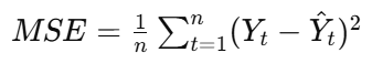
MSE

• mean squared error

• how well a model’s predictions match the actual data

• Yt​: actual value

• Y(hat)t​: predicted (forecasted) value

• n: number of observations

• (Yt−Y(hat)t): error (residual)

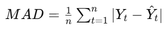
MAD

• mean absolute difference

• measure of the average size of forecast errors, without squaring them

• Yt​: actual value

• Y(hat)t: predicted (forecasted) value

• n: number of observations

• ∣Yt−Y(hat)tl: absolute error (ignores sign)

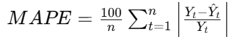
MAPE

• mean average percentage error

• measures forecast accuracy as a percentage

  • makes it easy to interpret across different scales

• Yt: actual value

• Y(hat)t​: forecasted value

• n: number of observations

• The fraction = percentage error for each observation

How do you choose the best forecasting model?

• MAE → average absolute mistake

• MSE → penalizes large errors more

• MAPE → percentage error

The lower, the better