Microeconomics

Reflexivity Assumption

• It is assumed that each bundle is at least as good as itself

Preference Symbols

Ad valorem tax and subsidy

• Ad valorem means 'to add value'

• An ad valorem tax means a tax is paid on a good based on its price; a subsidy implies the inverse

Budget Constraint

• The budget line is given by p₁x₁ + p₂x₂ = m, which just exhausts a persons income

• It has a slope of −⁡p₁/p₂, a vertical intercept of m/p₂, and a horizontal intercept of m/p₁.

• The Numeraire is when one of the variables is fixed as constant; this doesn't change the constraint (check by rearranging)

• Increasing income shifts the budget line outward. Increasing the price of good 1 makes the budget line steeper. Increasing the price of good 2 makes the budget line flatter.

Pareto Efficiency

• An allocation is Pareto Efficient if there is no way of making one better off without making another worse off

Equilibrium Principle

• Generally, prices are determined when supply for a good meets the demand for a good

Optimisation Principle

• People choose the best patterns of consumption available to them 

Endogenous and Exogenous Meaning

• Most simply, endogenous variables are explained and contained in a particular model whereas exogenous variables are not 

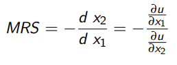
Marginal Rate of Substitution

• The rate at which an agent will swap one good for another

• The slope of an indifference curve

Monotonic Transformation

• Utility functions are ordinal, meaning they only show an order of preference, but don't assign an actual value to preferences

• If preferences are represented by numbers - coffee = 4 and tea = 5 - by adding 5 to the values the order of preference is preserved

Perfect Substitutes

• An agent is completely indifferent between two goods; they seek to maximise utility regardless of which good they have 

• u(x,y) = x + y

Perfect Complements

• When two goods are only enjoyed when consumed together; there is no point having more of one good without the other

• u(x,y) = min(x,y)

Convexity Assumption

• Averages are better than extremes

• This works when we take a weighted average of two bundles of goods and represent it on an indifference curve; this new curve will be equal to or strictly preferred to the singular curves

Transitivity Assumption

• A logical assumption which mitigates against preference cycles

• There is no situation in which A > B, B > C, and C > A

Monotonicity Assumption

• Assumes that more of a good is better

• This simply means that in models we will only study allocations of goods before satiation occurs

Completeness Assumption

• Agents are able to exhibit preferences, avoiding situations in which they can't choose between different bundles

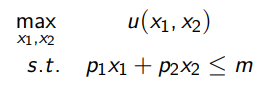
Marshallian Demand

• The solution to the constrained optimisation problem in the image 

• This solution gives the optimum quantity given fixed income and prices x(p,m)

The Equimarginal Principle

• Most utility curves are smooth and convex (Cobb-Douglas Equations)

• At the optimum, the indifference curve and budget constraint will be tangent at the optimum, giving the equimarginal condition

• Find the marginal utility by differentiating a utility function with respect to one of the arguments, then set the ratio of the marginal utilities equal to the ratio of the prices

• MU_x1/MU_x2 = x₂/x₁, x₂/x₁ = p₁/p₂

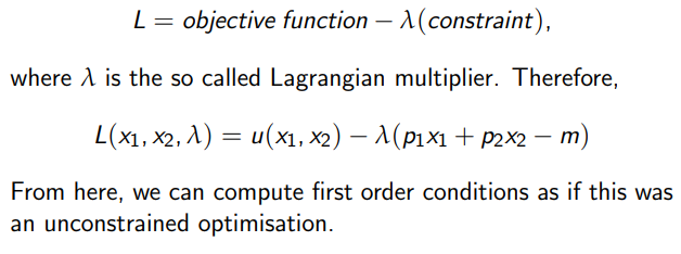
The Lagrange Method

Revealed Preference

• In a situation where there are two goods available and one chooses A over B, we can say that A is revealed preferred to B 

Weak Axiom of Revealed Preference

• If a person chooses x over y at some prices p when both are affordable, we can never reverse the choice at any other price in which both are affordable

• Thus, something consists with the weak axiom of revealed preference if someone has a strict preference of one good over another

Strong Axiom of Revealed Preference

• Adds a condition to the weak axiom which ensures that transitivity is respected

• If A is revealed preferred to B, and B is revealed preferred to C, then C can not be revealed preferred to A (this event would be lots of curves crossing each other)

Optimal choices for concave preferences

• Concave preferences imply a person doesn’t want to buy two goods together (like olives and ice cream; if they have ice cream they DON'T want more olives)

• Thus the solution for nonconvex preferences is always a boundary point

Shortcut for optimal choices in Cobb-Douglas

• To be used instead of conducting the Lagrangian, where the Cobb-Douglas is given by u(x₁,x₂) = x₁^cx₂^d

• It is often useful to choose Cobb-Douglas functions where the exponents sum to 1 because this means that the exponents can be interpreted as a fraction of income

Normal good

• A type of good where an increase in income will increase demand (eg cars, steaks)

• dx₁*/dm > 0

Inferior good

• As income increase, demand for the good decreases (eg fast food)

• dx₁*/dm < 0 

Ordinary good

• Demand decreases when price increases (eg clothes)

• dx₁*/dp₁ < 0

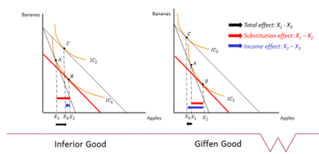
Giffen good

• Demand increases when the price increases (watches, cars)

• Often referred to as luxury goods; they are partly valued because of their price

• dx₁*/dp₁ > 0

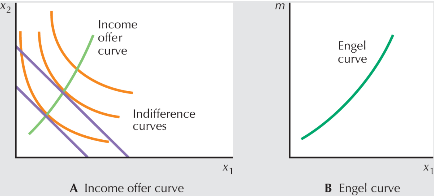
Engel Curve and Income Offer Curves

• The shape of the income-offer curve is referred to as the income-expansion path; when income increases and the goods are normal, the slope will be positive 

• The income offer curve illustrates the bundles of goods demanded at different income levels 

• The Engel curve is one which shows the path of demand for a good given fixed prices

Demand Curve

• Derived by plotting all of the price-demand combinations on a graph (price over demand)

• Shows how one person reacts to changes in price and income

Price Elasticity of Demand

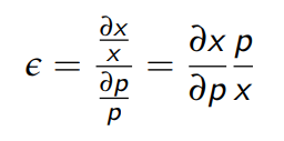
• The slope of a demand function, understood as the ratio of relative changes

• When the PED > 1, demand is called elastic, meaning that the demand curve is flatter (x changes a lot with price)

Constructing market demand

• Summing horizontally is equivalent to fixing the price and summing the demand of different consumers

• This allows one to find aggregate market demand at a particular price

• Kinks can occur when one is summating market demand and a price goes above one of the consumers WTP

Slutsky Decomposition

• Deals with the effects a price change has on demand

• The first effect is the substitution effect; a person switches consumption to the other good

• The second effect (income effect) involves a change in purchasing power

• This separating of these two effects is called the Slutsky decomposition

Compensated Demand 

• Is constructed to eliminate any purchasing power (income) effect 

• If original prices are p₁ and p₂, with income m, then when prices change to p₁’ and p₂, the new income must be m’ to allow for purchasing the same quantities at different prices 

Substitution effect

• When a person shifts consumption from one good to another after a price change

• The difference between the bundle x* and x’ (where x* is the original quantity demanded, and x’ is the quantity demanded after the price change)

• The solution to max_(x1,x2) u(x₁,x₂) s.t. p₁’x₁ + p_2×2 = m’

Income effect

• The loss of purchasing power caused by a price change, which is found by locating the optimal bundle at a new price and non-adjusted income

• We move from x’ (adjusted demand with adjusted income) to x’’ (adjusted demand with non-adjusted income)

• The income effect is the difference between x’’ and x’

• The solution to max_(x1,x2) u(x₁,x₂) s.t. p₁’x₁ + p_2×2 = m

• Graphically, this is a linear transformation of the budget constraint and indifference curve tangency 

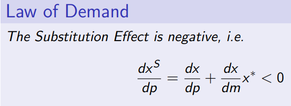
Slutsky Decomposition - Maths

• Where dx/dp is the change in demand w.r.t the change in price and x*(dx/dm) is the income effect

Homothetic preferences on Engel and Income Offer curves

• They will always be represented as straight lines through the origin, because any change in the quantity of bundles doesn’t change the ratio of preferences

Quasilinear indifference curves

• All the indifference curves are just linear transformations of one indifference curve 

• We say that there is zero income effect due to an increase in income, and the Engel’s curve is a straight vertical line 

The Price Offer Curve

• When we change the price of one good, keeping the other fixed, the budget constraint pivots, intersecting different indifference curves at different points

• These new intersections are connected through the price offer curve

Hicksian Compensated Demand

• Also known as the Hicksian Subsitution Effect, this computes the optimal point by fixing utility and finding the compensated demand required to reach this utility

• This implies a new solution framework; we can’t maximise the problem because we’re keeping utility fixed, so we invert it and solve in terms of expenditure minimisation instead

• We minimise expenditure using the Lagrangian or Equimarginal Principle

• min_x1,x2 p₁x₁ + p₂x₂ , s.t. u(x_1,x₂) = u*, where u* is the fixed level of utility

• The minimal point lies on the lowest budget line touching the indifference curve constraint 

Unconstrained Optimisation 

• Rearrange the budget constraint to get x2 = (m-p₁x₁)/p₂

• Substitute this into the utility expression and then maximise it, solving for x₁ by setting it equal to 0

Hicksian Demand Substitution Effect

• We want to fix utility at its optimal level, so plug the Marshallian demands into u(x₁, x₂) to find the optimal utility, u*

• Minimise expenditure subject to the new constraint (ie, x₁x₂ = u*) and compute 

• Solve for new optimal quantities given the price changes; take x₂ from x₂^* to see the substitution effect 

• These new optimal quantities, x₁^* and x₂^* are called Hicksian Compensated Demands, subject to H(P1, P2, v), where v is the fixed level of utility 

Hicksian Demand Income Effect

• Simple compute the Marshallian demands of the goods at the new prices; this accounts for what expenditure will actually be like given the change in income 

Hicksian Demand Total Effect

• The direction of the total effect depends on what type of good it is; for a normal good, the substitution and income effect will both be positive

Compensating Variation

• Fix utility before the price change and find how to adjust income to ensure the same utility after the price change

• If e(p’, u(x*(p, m))) is the minimum expenditure needed to achieve the same utility at final prices, then the compensating variation, CV (p,p’,m) = |m - e(p’, u(x*(p, m)))|

Equivalent Variation 

• Fix utility after the price change, u(x*(p’, m))

• Tries to figure out how we can adjust the income to ensure the consumer experiences the same level of utility before the price change as it does after 

• EV(p, p′, m) = |e(p,u(x*(p′, m))) − m|

Consumer Surplus

• The net benefit we receive from consuming q units of good 1, where CS(q₁) = v(q₁) - p₁q₁

• The area below the demand curve

Comparing Equivalent Variation and Compensated Variation

• For a normal good, CV > EV for a price increase and vice versa for a decrease

• They will only be equal for quasilinear preferences where indifference curves are parallel and there is no income effect

Computing Compensated Variation

• Original budget constraint is P₁*x₁* + P₂x₂ = E₁. When the price of P₁ rises to P₁**, the budget constraint changes with new Marshallian Demands to become P₁**x₁** + P₂×₂** = E₁

• We shift the second budget line out so that it becomes tangential to the original utility curve. The budget constraint becomes E₂ = P₁**x₁*** + P₂x₂*** where E₂ is compensated income

• E₂ - E₁ is the compensated variation

Computing Equivalent Variation

• How much money to take away from a consumer before a price change to ensure they will be just as well-off after it

• Original BC is P1*x1* + P2x2* = M1

• When the price P1 rises, BC pivots inwards and new BC is P1**x1** + P2x2** = M1

• We must takeaway money from the consumer to ensure constant utility, so shift the original BC inwards to get the new BC P1*x1*** + P2x2*** = M2

• EV = M1 - M2

How are demand functions given?

• In the form, x₁ = x₁ (p₁, p₂, m), as a function of both prices and income

The Slutsky Identity (for the total change in demand)

• x₁(p’₁, m) - x₁(p₁, m) = (x₁(p’₁, m’) - x₁(p₁, m) + (x₁(p’₁, m) - x₁(p’₁, m’))

• This is an identity, true for all values

• This could be simplified into easier symbols like; x’ - x = (x’’ - x) + (x’ - x’’), or x = x^s + xⁱ

• It is the addition of the substitution and income effect respectively

What is the graphical difference between Hicksian and Slutsky substitution effect?

• For the Slutksy substitution effect, the budget line pivots around the optimal point to show the effect

• For the Hicksian substitution effect, the budget line doesn’t pivot around the optimal point, but instead moves around the original indifference curve to reach a point which has the same gradient as the final budget line

  • Thus, where Slutsky keeps purchasing power constant, Hicks keeps utility constant

What is uncertainty?

• Uncertainty concerns missing information, where the link between cause and consequence, choices and outcomes, is not clear

Risk

• This is where an agent knows the achievable outcomes and probabilities of achieving those outcomes rather than simple uncertainty

Expected outcomes (and utility)

• Involves multiplying the outcome of a situation by the probability that it happens 

• Expected utility involves attaching a utility weight to an outcome; in the case of a lottery, it might look like EU(w) = p₁ux₁ + p₂ux₂, where u = utility, p = probability, EU(w) is expected utility of wealth, and x is an outcome

Certain Equivalent 

• This is the concept of the certain lottery which is equivalent to the risky one 

• This is the amount of money it would take for a person to be indifferent between the certain amount and the uncertain lottery (the ‘riskier’ choice)

• u(CE) = EU(w) = pu(w1) + (1 − p)u(w2)

Risk attitudes

• Risk averse | CE < E(w), EU(w) < u(E(w)) — This basically means that the expected utility of the wealth is less than the utility of actually having it; they have more utility by not taking the risky lottery

• Risk neutral | CE = E(w), EU(w) = u(E(w))

• Risk lover | CE > E(w), EU(w) > u(E(w))

What is Insurance?

• Insurance is effectively trading risk; a person would prefer to pay some amount in the eventuality that they are faced with a bad state (lose their car, etc)

Optimal Insurance Contract

• k is the amount ensured, w is the value of the insured object, A is the potential damage, á is the price per pound insured, p is the probability of the damage-causing event 

• Thus, expected utility maximising equation is max_kEU(k) = (1 − p) u(w − αk) + pu(w − A + (1 − α)k)

Insurance FOC

• dEU(k)/dk = α(1 − p)u′(wg ) − (1 − α)pu′(wb) = 0

• (1 − p) u′(wg) / pu′(wb) = (1 − α) / α

• Full insurance, or constant wealth, only occurs when k = A

• To make insurance optimal, we must have that p = α, to ensure a ‘fair price’

Willingness to pay and risk premium

• An agent is only willing to pay the difference between wealth in the good outcome and the Certain Equivalent

• The risk premium is the amount an agent is willing to pay with respect to a risk neutral person, quantified by the difference between E(w) and the Certain Equivalent

Adverse Selection

• Involves the situation when two people enter a contract with asymmetric information; a risky driver who should pay a higher insurance premium tries to enjoy lower insurance prices by hiding their behaviour

• This is also called a ‘hidden characteristic’ or ‘hidden information’ problem

• This could lead to non-efficient outcomes or even stop trading in some markets

Moral Hazard 

• Occurs when someone has no incentive to mitigate risk because they’re completely insured

• In the case of bicycle insurance, a person might not take any care at all if they are reimbursed completely for losing it because they have already made the investment in insurance (as opposed to investing in a really heavy and secure bike-lock)

• Occurs when one side of the market can’t observe the actions of the other — a hidden action problem 

Signalling

• A way to try and solve the ‘lemon market’ problem; sellers can offer warranties to insure a consumer against the risk of their car being a lemon

• Owners of the good cars can afford this whereas the owners of the bad cars can’t

The Incentive Compatibility Constraint

• Simply states that the utility to the worker of some effort level x* must be greater than any other effort level; this effort level is the one which maximises profit for the incentiviser

• Marginal cost of effort must be equal to the marginal product of effort

• The incentiviser can aim to do this through many ways:

How might a landowner incentivise a worker in line with the incentive compatibility constraint?

1. Rent (rent the land to the worker, they keep all the profit over the amount they pay back to the owner)

2. Wage labour pays a person an hourly rate

3. Take-it-or-leave-it: the worker is paid if they work at x* and nothing else

4. Sharecropping is where the owner and worker both take a percentage of the product of labour

What is the independence assumption?

• It is the idea that consumption patterns in one state are independent of another state; how much money I am willing to sacrifice in order to get a little more money if my house burns down should be independent of the event that my house doesn’t burn down

• Thus, expected utility functions must have an additive form (like p₁c₁ + p₂c₂) to ensure that they are independent

What is expected value of wealth?

• In a situation with uncertain outcomes, the expected value of wealth, or the utility of expected wealth, is given by finding the average value of the two outcomes

• If we have a 50% probability of getting $5 and $15 respectively, then the expected value of wealth is the average of 5 and 15: $10

• The utility of expected wealth is u($10)

• This is given by ½ (5) + ½ (15) = 10

What is the expected utility of wealth?

• In the situation where there are uncertain outcomes, a 50% probability of receiving $5 or $10 respectively, the expected utility of wealth is found by calculating the sum of the two expected utilities

  • Note that this calculates expected utilities rather than expected wealth

• Given by ½ u(5) + ½ u(15)

What are the shapes of risk-averse and risk-lovers utility functions?

• The risk-averse consumers utility function is concave whereas the risk-lovers graph is convex (increasing gradient)

• Utility on the y-axis, wealth on the x; these different functions show that a persons preferences ‘lean’ towards the axis they value more

A pure exchange economy

• Aim to describe an economy through simple concepts

• We need three objects, a set of traders, preferences, and resources (each agent is given some endowment)

• Generally we’ll use the simple framework of two agents and two goods

The Edgeworth Box

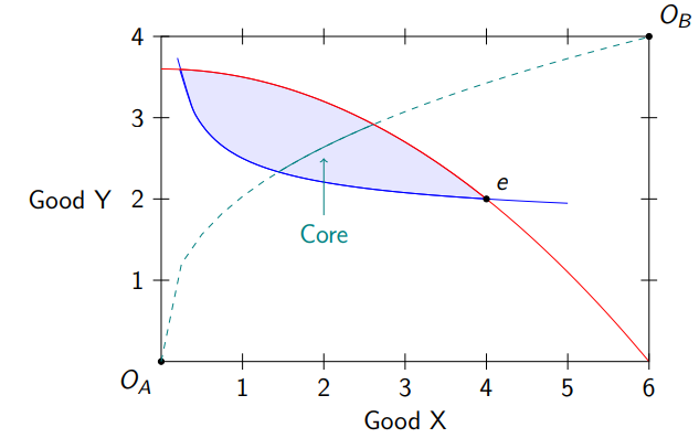
• Consists of fitting the different indifference curves of the different agents into the same graph, from opposite origins, where the sizes of the edges represent the total resources in the economy

• There are equilibrium trades where the indifference curves intersect

The contract curve

• Is on the same Edgeworth box as the other utility curves, and is the set of all possible Pareto efficient allocations 

• The set of Pareto efficient allocations which improve upon the original endowment is called the core 

Allocation in competitive markets 

• The main mechanism for allocation is price, meaning individuals simply maximise where their income is the value of their endowment (endowment is valued in monetary terms)

• A competitive equilibrium occurs when there is an allocation that maximises each person’s utility at a set of prices (they are price-takers) and the market clears 

• On the Edgeworth box, the difference between the original equilibrium and the competitive equilibrium can be conceived of in terms of an agents excess supply and excess demand 

What is the first fundamental theorem of welfare?

• Competitive equilibrium allocations are Pareto Efficient

• Requires some monotonicity of preferences as an assumption

• This tells us that a competitive economy will end up at some point on the contract curve; a lump sum transfer is a way of transferring money to change the initial endowment and end up on a better place on the contract curve

What is the second fundamental welfare theorem?

• For each efficient allocation on the contract curve, there is a price that supports it as a competitive equilibrium 

• The results requires convexity of preferences and tells us what we can achieve with redistribution 

• Every point on the contract curve can be reached through decentralised trade

What are political implications of the welfare theorems?

• Markets can produce good results

• Perfectly competitive markets provide the benchmark

• Government redistribution can help ease ethical concern within the market

The second theorem and lump sum transfers

• The second theorem assumes we can do lump sum (costless and immediate) transfers (presumably done by the government through taxation)

• This taxation can still lead to an equilibrium market outcome so long as the thing being taxed can be measured or can’t be changed (taxing people with blue eyes’ endowment and giving it to people with brown eyes. Or, taking from people with High IQ’s endowment and redistributing it to lower IQ endowments)

  • This works because we recognise that all trades which occur from initial endowments will result in a Pareto efficient market equilibrium

Situations in which markets are inefficient

• Market power: there are agents big enough to be price-makers rather than price-takers

• Externalities, where one individuals welfare depends on the consumption of others 

• If information is incomplete, trading might be obstacled leading to inefficiency 

• The pricing of public goods by private sectors doesn’t result in efficient allocation 

What is gross demand?

• Gross demand is the total amount of a good that a person wants to consume at the going price

What is net demand?

• This is the difference between gross (total) demand and the initial endowment they already have

  • It is how much the consumer needs to buy of the good to satisfy their demand of the good

What is Walras’ Law?

• It is a condition which specifies that in equilibrium, the value of the aggregate excess demand in an economy is identically equal to 0

  • p₁z₁(p₁, p₂) + p₂z₂(p₁, p₂) = 0

• This identity means that the value of aggregate excess demand is necessarily 0 for all prices, not just those in equilibrium; it is stronger than necessary

Relative prices

• Walras’ law demonstrates that in a market with k goods, we only need to find prices for which k-1 markets are in equilibrium; the k^th market will necessarily be in equilibrium

• It seems that we are unable to solve for the final price because we have k goods and only k-1 equations, but this is because the k-1 equations are only solving for independent prices

• Thus we need to fix a price as constant so that all other prices can be measured relative to it

What is Arrows’ Impossibility Theorem?

• If a social mechanism satisfies certain properties (1. the decision mechanism should be complete, transitive, and reflexive, 2. everyone should rank x ahead of y if everybody prefers x to y and 3. that preferences between x and y should depend only on how people rank x versus y and not on other preferences) then this social decision-making mechanism is a dictatorship

  • This just means that this mechanism for choosing between pareto efficient outcomes resembles the preferences of just one person, not many

• If we want to aggregate social preferences whilst maintaining democracy, we will have to give up one of the three properties that are listed in Arrow’s impossibility theorem

When is an allocation equitable?

• An allocation is equitable when a person doesn’t prefer any bundle over their own allocation

• To desire another persons bundle is to envy it

• We say that if an allocation is equitable and pareto efficient, then it is a fair allocation

Why does a market fail?

• Due to agents not being price-takers, the market is unable to arrive at efficient outcome due to the pricing mechanism

Simple monopoly model

• A single firm with a cost structure c(q) is facing an inverse demand curve p(q)

• The firm maximises p and q for π(p,q) = pq - c(q) s.t p = p(q)

  • By incorporating the constraint, one can just maximise π(q) = p(q)q - c(q)

• The solution to this gives the marginal revenue, equal to the marginal cost, which is dc(q)/dp

• This leads to a deadweight loss in the market

What is a game?

• Requires a set of players, sets of strategies, timing, information, and payoffs

• A game has these features

What types of games are there?

• Cooperative and non-cooperative games

• Simultaneous and sequential games

• Complete information and incomplete information 

  • We might also include one-shot and continuous games

What is normal form?

• The simplest way of representing a game and its outcomes 

What is a dominant strategy?

• A strategy which is best for one player regardless of what their opponent chooses

Nash Equilibrium

• When players play their mutual best responses

• It also requires the absence of regrets; upon knowing what your opponent is doing you do not change your mind

Entry deterrence

• Suppose a sequential game where a firm is enjoying a monopoly

• Another firm wants to enter the market; the firm in monopoly might decide to react heavily or lightly to this; they might perform an action which doesn’t provide them with the greatest monetary value but it discourages others from entering the market 

• In sequential games, games are represented by trees

Strategies in sequential games

• A strategy is redefined as the set of actions a person undertakes at every node

• This means that in the sequential game, where the second player responds to the first, although the first only makes one decision, the second persons best strategy is to act conditionally on the first

• This allows for an expanded normal form

A non-credible threat

• A threat of adopting a particular strategy which has no weight because the actor would want to deviate from it once it gets to their turn in the game

What is a subgame?

• It is a part of sequential games and can standalone as its own game; it has well defined players, strategies, payoffs etc

• These games can have their own Nash equilibria — subgame perfect nash equilibria 

What is subgame perfect nash equilibrium?

• The set of strategies which constitutes a nash equilibrium in all the subgames

• To compute this we use backwards induction, which involves deciding what the first player will choose given the decisions of the subsequent players