Topic 1: Digital Signals and Systems

Advantages of digital signal processing

• Flexibility

• Programmability

• Repeatability

• Stability

• Data compression

• Cost

Flexibility detail

• Data can be sampled in real-time, and if necessary, readily processed offline at some later date.

• Since the data is stored digitally (no-volatile), the data can be applied to many different algorithms in order to find the most appropriate for a particular application.

• Algorithm complexity is largely limited only by available memory space and processor speed, and algorithms can be readily made automatically adapt to the surrounding environment.

• Some very useful algorithms are specifically derived for the discrete-time domain, and have no analogue-domain equivalent.

Programmability detail

• Many digital signal processors are now available which can be readily reconfigured to perform a multitude of different signal processing tasks.

• A change in software is all that is necessary to accommodate a different algorithm.

• Hardware re-development costs are minimal. It also means that a minimum number of discrete components are required to implement very complex
  processing algorithms

Repeatability detail

• Since digital systems are configured by software or external digital hardware, the functions that they perform are very repeatable

Stability detail

• Storage and processing of data by digital hardware means that problems associated with analogue processing, are not encountered.

Data compression detail

• Information channels for data transmission over long distances can be very expensive. Compression can:

  • Lead to less information needing to be transmitted

  • Ensure that all the valuable information held in the original data can be reconstituted at the receiver.

Cost detail

• The application of digital signal processors in becoming increasingly widespread, and hence, in many cases, the cost of digital algorithm implementation is less than analogue equivalents.

Normalised frequency

Cycles / sample or radians / sample

f_n = f / f_s w_n = 2 * pi * f_n

Properties of Digital Signals

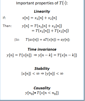
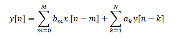
Linear Constant Coefficient Difference equations

Causal LTI systems can be described by a difference equation

Impulse response

• The impulse response of an LCCD system is denoted with h

• The response of the system to a unit impulse

• The output of the system 𝑇 when it is fed an impulse 𝛿[𝑛] is exactly the impulse response, ℎ[𝑛]:

Impulse response properties

• An LTI system is Bounded Input Bounded Output stable provided the sum of the impulse response is less than infinity

• An LTI system is causal provided the impulse response is 0 for all values of n < 0

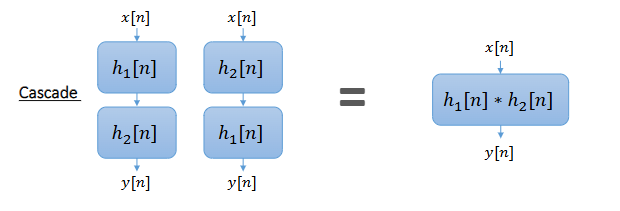
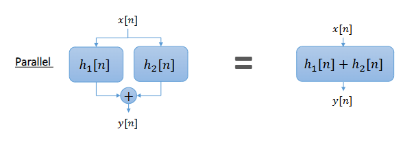
• Convolution is commutative and distributive

Parallel systems

Cascade systems