Microeconomics

Define microeconomics as a field of study.

Microeconomics is a Branch of economics that deals with the behaviour of individual economic units—consumers, firms, workers, and investors—as well as the markets that these units comprise.

Explain the difference between positive and normative analysis.

Positive - objective, fact-based, can be tested. Normative - subjective, value/opinion-based, cannot be tested.

Explain what the market is.

A collection of buyers and sellers that together through their actions (actual or potential) determine the prices of the goods.

Mrket mechanism

A tendency in a free market for a price to change until the market clears

Supply and demand curves equations

Q_d = a - bP (a - y-intercept, b - slope = dQ_d/dP) Q_s = c+dP

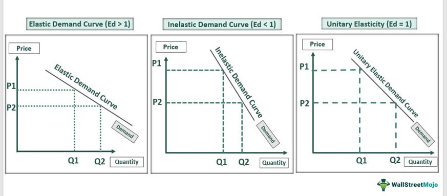
Price elasticity of demand/supply formula + analysis

E_QdP = dQ_d/dP * P/Q_d

• >1 → elastic

• =1 → unit-elastic

• <1 → inelastic

(considering absolute values)

Explain

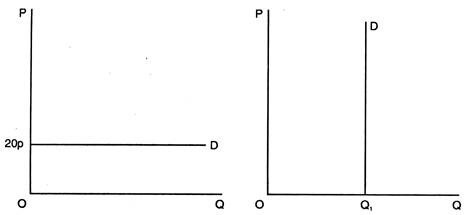
a) Horizontal or Perfectly Elastic demand (E=infinity)

b) Vertical or Perfectly Inelastic demand (E=0)

Income elasticity of demand formula + analysis

E_QdI = dD/dI * I/D

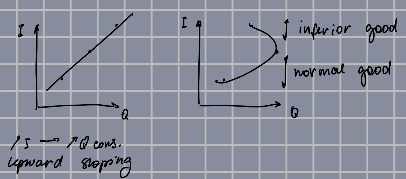
• >0 → normal good

  • >0<1 → necessary good (1>E>0 )

  • >1 → luxury good

• <0 → inferior good

Cross - price elasticity of demand formula

E_QdxPy = dQ_dx/dP_y * P_y/Q_dx

Point vs Arc elasticity

Point - at a certain price point on the curve

Arc - over a range of prices

Short run vs Long run

Short run: L variable, K fixed (more than 1 production factor cannot be changed)

Long run: L variable, K variable

Durable goods

Goods for which income elasticity is larger in the short run than in the long run (for most goods the opposite, eg gasoline vs cars)

LTV vs Subjective theories

Value of the good is based on:

• LTV: socially necessary labour (L+K+Equipment etc)

• Subjective: individual consumer’s needs and attitudes towards the good

Marginal utility + formula

Additional utility (satisfaction) from consuming one additional unit of the good

MU_x = dTU/dX

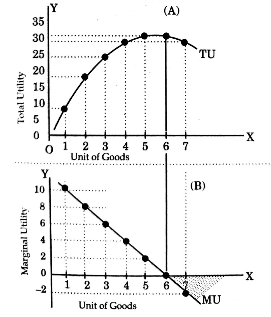
What is the slope of the total utility curve?

Marginal utility

Theory of consumer behaviour definiton

How consumers allocate incomes among different goods and services to maximise resources and satisfaction

TCB Assumptions

1. Completeness - consumers can compare all the alternatives

2. Costs are ignored

3. Transitivity - if A>B and B>C the A>C

4. Goods are desirable - more is always better than less

Goods for which less in preferred

Bads / Undesirable goods (eg pollution)

Indifference curve

A curve representing all combinations of market baskets that provide a consumer with the same level of satisfaction

IC Characteristics

1. Cannot intersect

2. U3>U2>U1

3. Negative slope → decrease Y to increase X

4. Convex curve

MRS

Marginal Rate of Substitution = maximum amount of a good that a consumer is willing to give up in oder to obtain one additional unit of another good (staying at the same level of utility)

MRS = MUx/MUy

What is the slope of the indifference curve?

MRS

Perfect substitutes

2 goods for which MRS of one for the other is a constant → straight line

Perfect compliments

2 goods for which MRS of one for the other is 0 (or infinite) → 90* angle bound lines

Utility

Numerical score that represents the satisfaction that a consumer gets from a certain market basket

Ordinal vs Cardinal utility

• Ordinal → general rankings from most to least preferred

• Cardinal → concrete numbers (by how much)

Budget constraints

Constraints that consumers face as a result of limited incomes

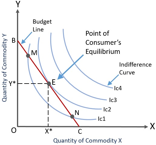
Budget line + equation formula

All combinations of goods for which the total amount of money spent equals income

I = Px*X + Py*Y

Slope of the budget line

Px/Py

Budget line intersect points with Y- and X-axis formula

• Y → I/Py

• x → I/Px

Consumer equilibrium equation formula

• MUx/Px = MUy/Py

• MUx/MUy = Px/Py

• MRS = Px/Py

• Slope of the indifference curve = Slope of the budget line

Marginal benefit

Benefit of consuming one additional unit of a good

To increase MUx..

We need to decrease X (amount of X) and vice versa

PCC

PCC = Price Consumption Curve = curve tracing the utility-maximising combinations of 2 goods that a consumer can buy at some price point (related to change in price of good X)

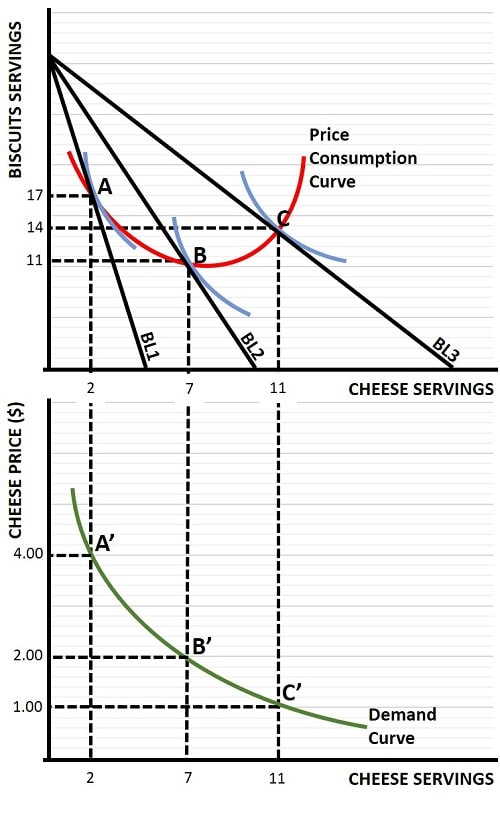
Demand curve can be drawn from..

PCC and MUx

Engel curve (ICC)

Curve relating the quantity of a good consumed to income

Isoelastic curve

Has the same elasticity at any point

Consumer surplus

The difference between the amount a consumer is willing to pay and the amount actually paid

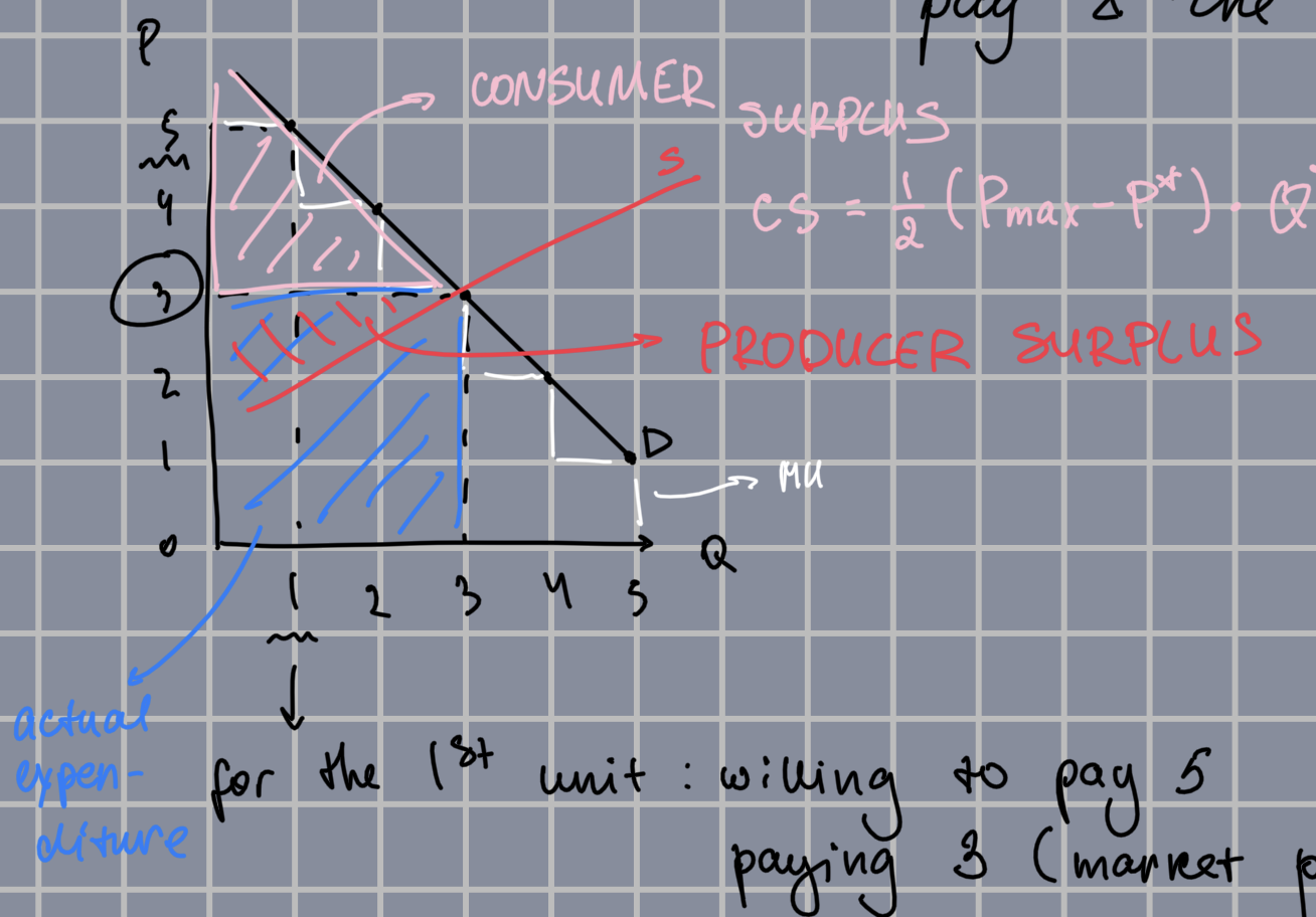
CS formula

((Pmax - P*) * Q*) / 2

Theory of the firm

How a firm makes cost-minimising production decisions and how the resulting cost varies with output

Factors of production

Inputs into the production process (labour → no of workers/hours, capital → machinery/buildings/materials/equipment - NOT money)

Production function

function showing the highest (fully efficient) output that a firm can produce for every specified combination of inputs

Efficiency

use of all resources in producing any give output (incl. personal time and energy)

Effectiveness

The degree to which the goals are achieved and/or the problems solved

Cobb-Douglas production function formula

Q = A*L^b*K^a

• A - degree of technology

• b and a - elasticities

Fixed input

Production factor that cannot be changed

Average product + formula

Output per unit of a particular input

AP_L=Q/L

Marginal product + formula

Additional product per one additional unit of input

MP_L=dQ/dL

Output elasticity formula

E_QL=MP_L/AP_L (dQ/dL * L/Q)

Inflection point, MP is..

max

+ returns increase not progressively but degressively

Short-run production graph

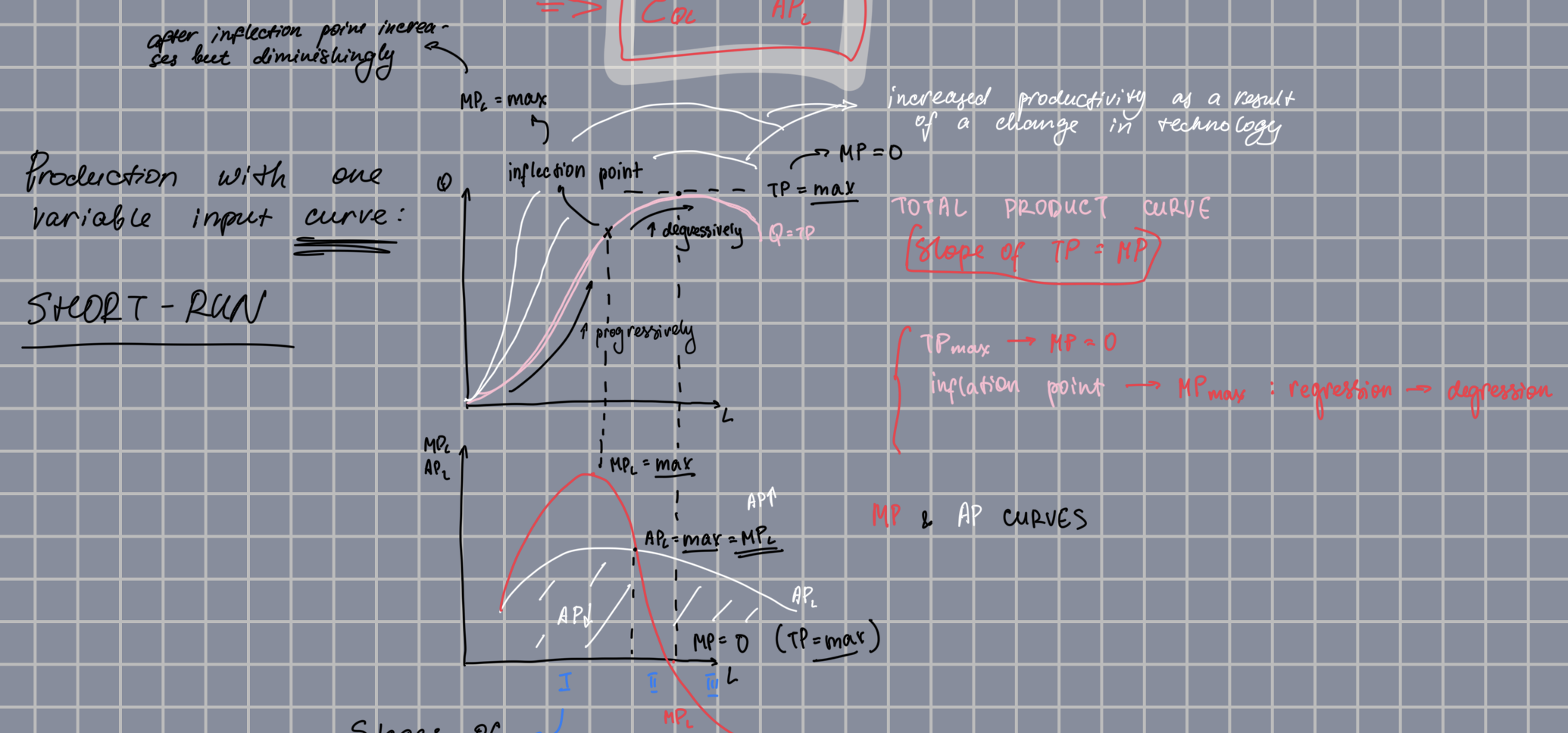
Sloope of the TP (total product) curve

MP

When TP is max, MP is..

0

When AP is max, MP is..

= AP

Stages of production

1. Stage of increasing returns: TP increases progressively, MP_L > AP_L and MP_K > 0

2. Stage of diminishing returns: starts at the point of AP_L = max = MP_L → TP increases degressively, MP_L < AP_L and MP_K > 0 but decreses

3. Stage of negative returns: starts at TP = max (MP_L = 0) → TP decreases, MP_L < AP_L and MP_K < 0

Law of diminishing marginal returns

As the use of an input increases (with other inputs fixed) the resulting additions to the output will eventually decrease

APPLIES ONLY TO THE SHORT-RUN PRODUCTION

Isoquant

Curve showing all possible combinations of inputs that yield the same quantity

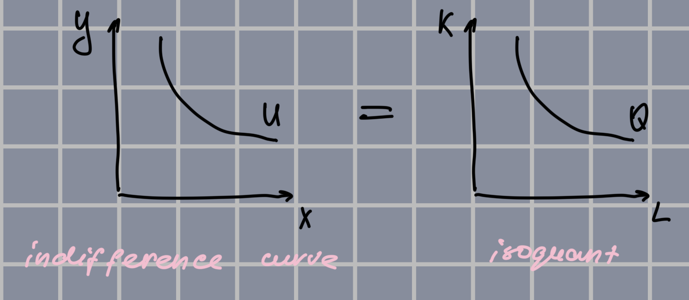
Slope of the isoquant

MRTS

Isoquant properties

• Negative slope

• Convex

• Cannot intersect

• Q3 > Q2 > Q1

MRTS

Marginal rate of technical substitution = the amount by which one input can be decreased to use one extra unit of another input to maintain the same level of production

MRTS formula

MRTS = MP_L/MP_K (=dK/dL)

Isocost

Curve showing all the different combinations of inputs that can be purchased for a given cost

Slope of the isocost

w/r

Producer equilibrium formula/equation

• MP_L/w = MP_K/r

• MP_L/MP_K = w/r

• MRTS = w/r

• Slope of the isoquant = Slope of the isocost

Perfect substitutes (inputs)

2 inputs for which MRTS of one for the other is a constant → straight diagonal line

Perfect compliments (inputs)

2 goods for which MRTS of one for the other is a constant = fixed proportions production function → straight angle bent lines

Returns to scale definition

Rate at which output increases as inputs are increased proportionately

Returns to scale types

• Increasing: input x2, output x>2 → lines closer to the origin

• Constant: input x2, output x2

• Decreasing: input x2, output x<2 → lines farther from the origin

PPF

Curve showing the various combinations of 2 different products that can be produced with a given set of inputs

Opportunity cost

Sacrificing the production of one good to produce more of the other

Slope of the PPF

MR(P)T

MRT

Marginal rate of (product) transformation = the rate at which one product must be sacrificed in order to produce a single extra unit of another product

MRT formula

MRT = MC_A/MC_B

Optimal production point formula/equation

• MC_A/P_A = MC_B/P_B

• MC_A/MC_B = P_A/P_B

• MRT = P_A/P_B

• Slope of the PPF = Slope of the isorevenue line

Slope of the isorevenue line

P_A/P_B

Economies of scope

When the joint output of a single firm (2 products) is greater than the output that could be achieved by 2 different firms (1 product each)

Returns to scale formula

RTS = Eq,l + Eq,k

Marginal cost formula

MC = dVC/dQ = w/MP_L

Accounting cost

Actual expenses + depreciation of equipment

Economic cost

Cost of utilising economic resources including opportunity cost → Economic c. = Accounting c. + Opportunity cost

Amortisation

Treating a one-time expenditure as an annual cost spread out over some number of years

MC definition

Additional cost of producing one extra unit of output

Economies of scale

A situation in which output can be doubled for less than a doubling of costs

Cost-output elasticity formula

Etc,q = dTC/dQ * Q/TC = MC/ATC

Classifications of market structures (authors)

• Stackelberg (9 types, output market and input market)

• Samuelson (3 types: PC, limited competition (3 types), monopoly

• Waud (4 types)

• Weintraub (!)

In which market structure is product differentiated?

Monopolistic competition

Elasticity in different market structures (how graphs look)

• PC: E = infinite, Cross-Elasticity = 0

• M: E = small number, CE = 0

• O: E = infinite, CE = higher number

• MC: E = higher number, CE = small number

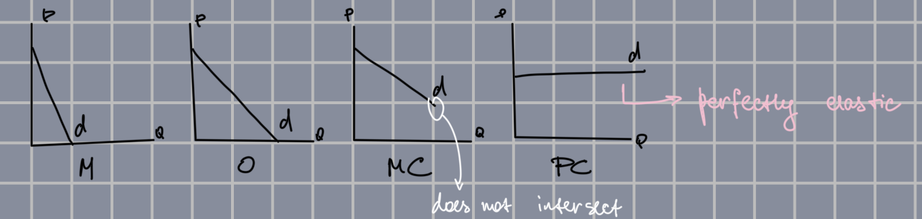
PC assumptions

• firms are price takers

• price = market price

• products are homogeneous and perfect substitutes

• free entry and exit

• P = MR = AR = d = MC

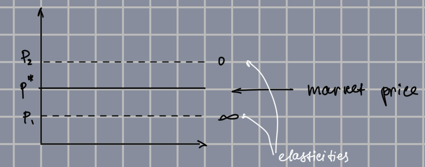
Accounting profit

TR - TC (EXCL opportunity cost)

Economic profit

Accounting profit - opportunity costs

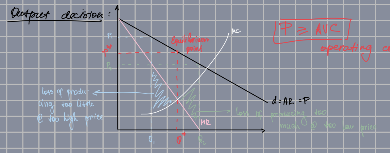
Profit maximisation/Output rule (2 conditions)

1. MR + MC (in PC → P = MC)

2. MR’ < MC’ (slope of marginal revenue < slope of marginal cost)

Marginal revenue

Change in revenue resulting from a one unit increase in output

Operating condition

P ≥ AVC

Supply curve

Marginal costs curve that is above AVC (ATC) in the short (long) run

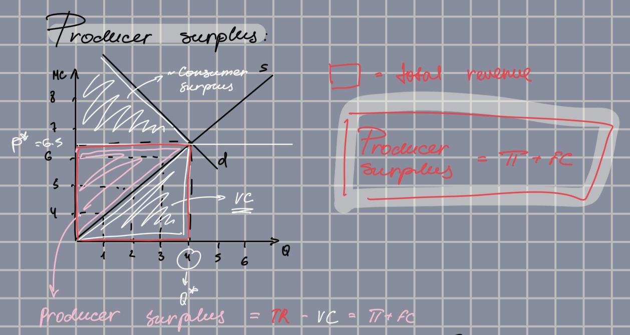
Producer surplus formula

• PS = TR - VC = PROFIT + FC

• It is above the MC curve and below the P*

• In LRPC PS = 0!

Monopoly

Market structure with only one seller selling a product without close substitutes (eg. water supply in a city managed by the givernment)

Monopsony

Market with only one buyer → input market

Market power

Ability of a seller or buyer to affect the price of a good

Average profit formula

Avg profit = AR - AC = P - TC/Q

Output decision graph