S2 L6 Panel data

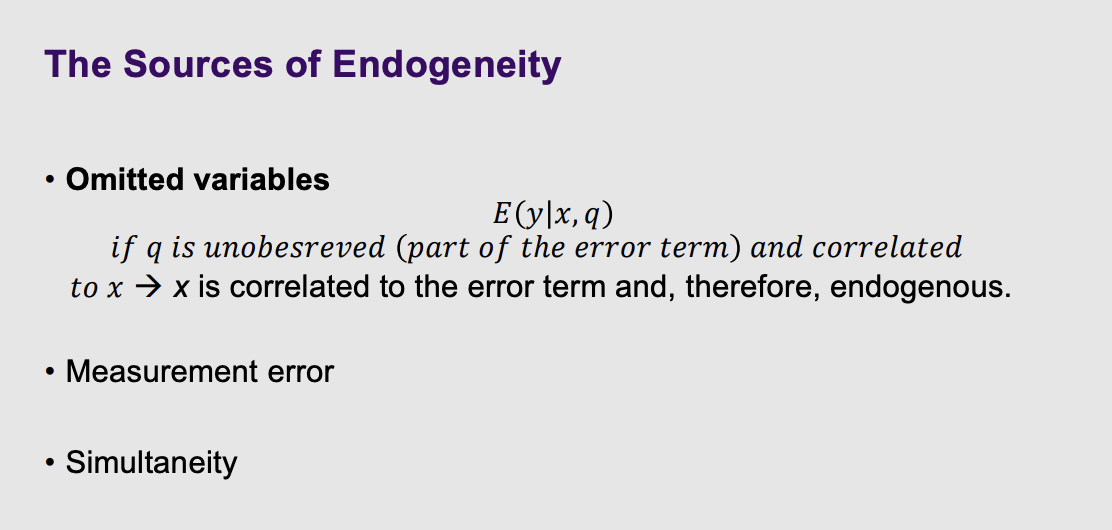
What are the sources of endogeneity

• What it means: This is a quick recap of the "villain" of econometrics: Endogeneity (when your data is mathematically contaminated).

• The 3 Causes: The slide lists the three main reasons this happens:

  1. Omitted Variables: You forgot to measure a hidden factor (like innate ability), so it secretly drives your results.

  2. Measurement Error: Your data contains typos or survey lies.

  3. Simultaneity: A chicken-or-the-egg feedback loop where $X$ causes $y$, but $y$ also causes $X$.

If one of the variables is correlated with the error term - Endogeneity

 

Don’t always have the luxury of longitudinal data, which is less prone to endogeneity.

 

What opportunities we have with panel data to remove the endogeneity.

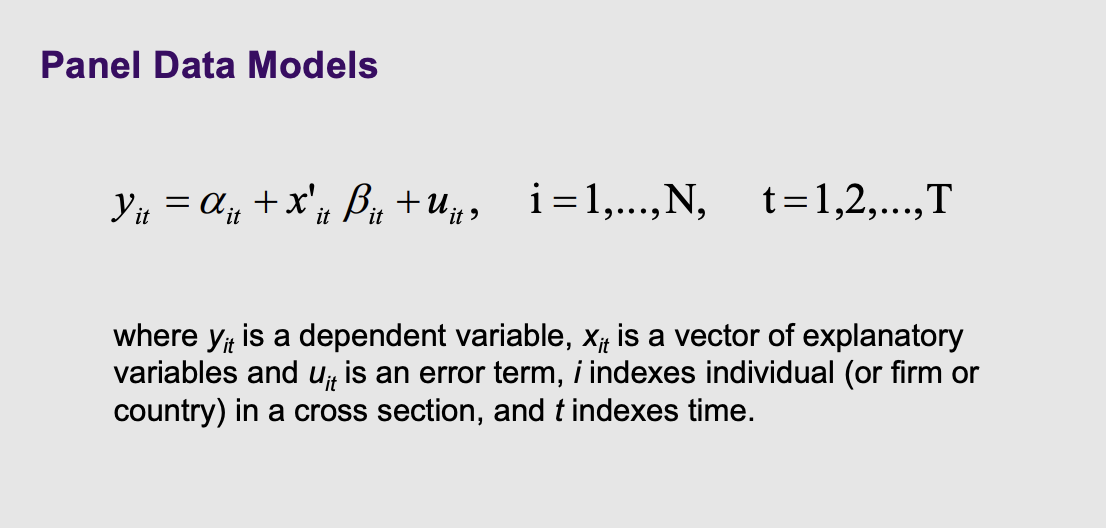
What does a panel data model look like

Sub script of the varibales at which dimensions vary. It under the variables means individuals across time

What it means: This introduces the basic formula for Panel Data: $y_{it} = \alpha_{it} + x'_{it}\beta_{it} + u_{it}$.

The Plain English Translation: Notice the little $i$ and $t$ subscripts attached to everything.

• $i$ represents the specific individual (or firm, or country).

• $t$ represents the specific year (or month, or day).

• Instead of just asking "What is John's income?", you are now asking "What is John's ($i$) income in the year 2010 ($t$)?".

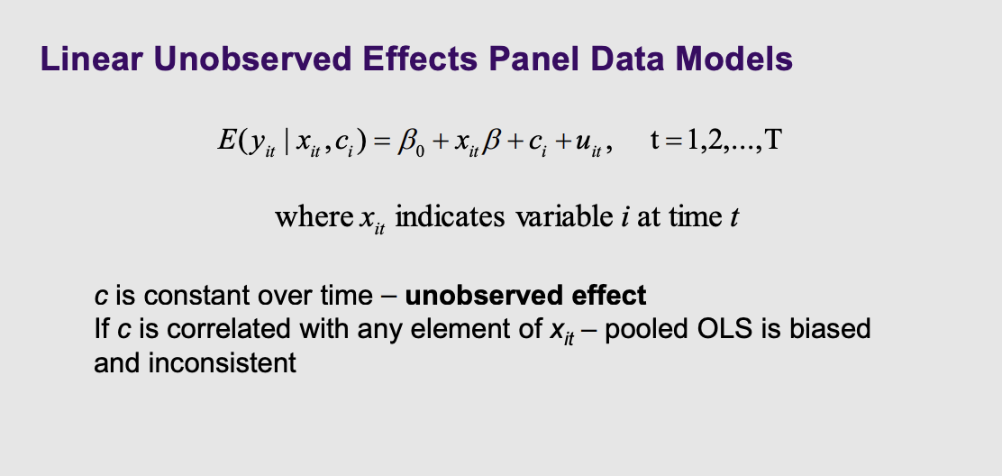
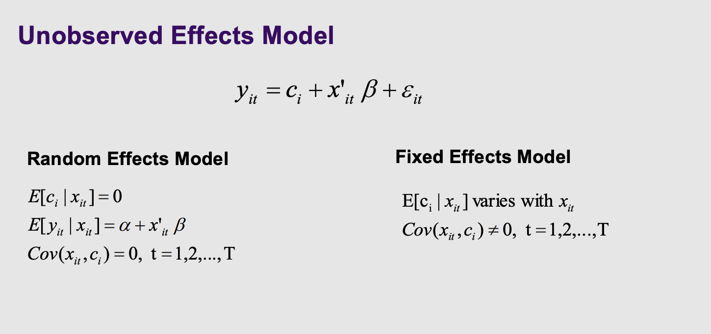
How are linear unobserved effects modelled in panel data models and what is the intutition of c

• What it means: The professor introduces a new mathematical variable into the equation: $c_i$.

  The Plain English Translation: $c_i$ stands for "unobserved effect" that is constant over time. Think of this as a person's permanent, unchanging hidden quirks—like their baseline personality, genetics, or the culture of the country they were born in. The slide warns that if these hidden quirks ($c_i$) are secretly correlated with the choices a person makes ($x_{it}$), standard math (Pooled OLS) will fail and give you biased answers.

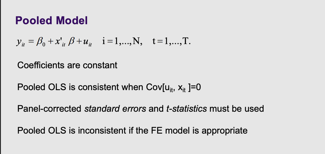
What is the pooled model and (4)

• What it is: This is the most naive model. It takes all the data across all years and throws it into one giant pool .

• The Problem: It pretends that getting 5 years of data from 1 person is the exact same thing as getting 1 year of data from 5 different people. It completely ignores the fact that a person's choices in 2010 are highly correlated with their own choices in 2011. To use this, you must use "panel-corrected standard errors" to fix the math, but it is often inconsistent .

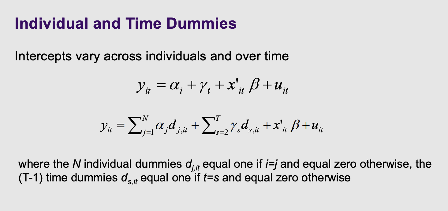
Individual and time dummies

• What it is: Instead of one single starting line for everyone, this model gives every single person (and every single year) their own unique mathematical intercept (starting line) .

  The Problem: If you have 10,000 people in your dataset, the computer has to estimate 10,000 different dummy variables ($d_{j,it}$), which exhausts the computer's calculating power .

What are the two unobserved effects models

• This slide introduces the two main heavyweight champions of Panel Data: Random Effects (RE) and Fixed Effects (FE) .

• The choice between them comes down to one single question: Are a person's hidden, unchanging quirks ($c_i$) correlated with the variables you are measuring ($x_{it}$)?

If YES: You must use Fixed Effects.

If NO: You can use Random Effects.

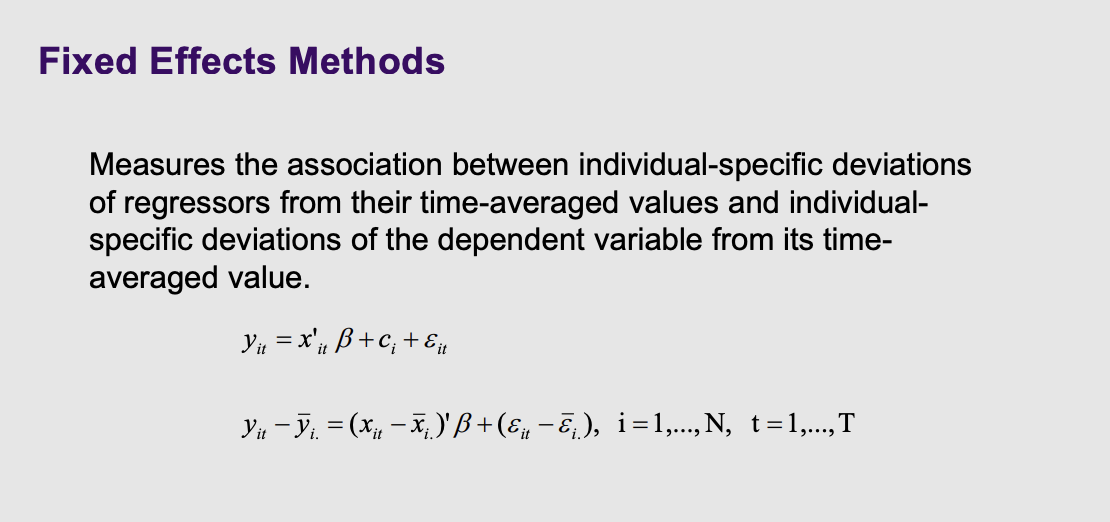
What is the fixed effects method

• What it is: The Fixed Effects model uses a genius mathematical trick to delete a person's permanent hidden secrets.

• How it works: Look at the formula: $y_{it} - \overline{y}_{i.}$. The computer calculates your average income over a decade, and subtracts it from your income this specific year. By only looking at deviations from your own personal average, anything that never changes (like your baseline genetics or race) gets mathematically zeroed out and deleted . The contamination is gone!

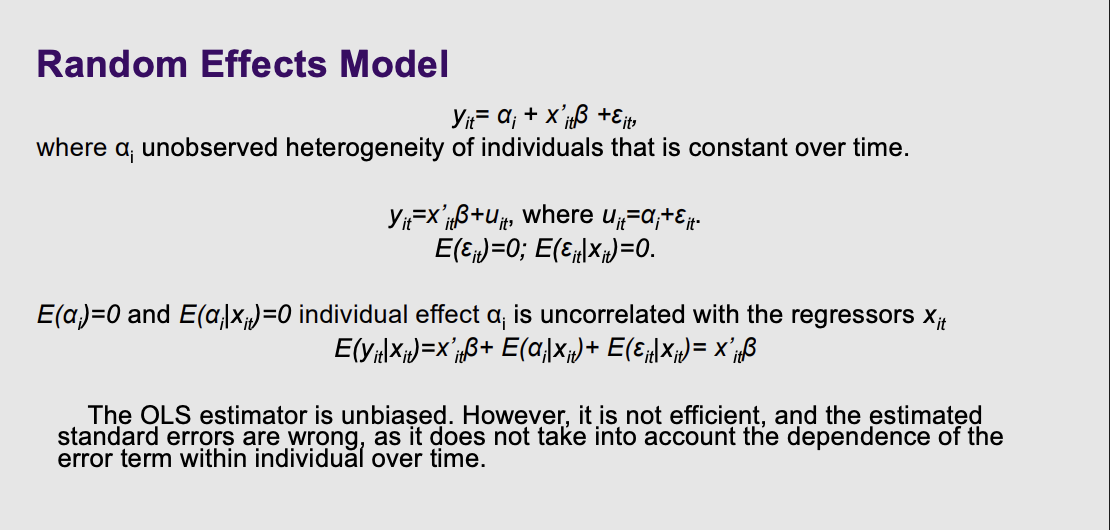
What is the random effects model, what is the alpha and what is the golden rule for random effects

• $\alpha_i$ (The Hidden Quirk): The slide calls this "unobserved heterogeneity... constant over time". As we discussed, this is the permanent baggage a person brings with them, like their innate ability or genetics.

• $\varepsilon_{it}$ (The Random Noise): This is the truly random, unpredictable stuff that happens year to year (like getting sick on the day of a test).

The slide then groups them back together into one giant error term: $u_{it} = \alpha_i + \varepsilon_{it}$.

2. The Golden Rule of Random Effects (The Middle Section)

This is the most important part of the slide:

$$E(\alpha_i | x_{it}) = 0$$

• What it means: The slide explicitly states that the individual effect ($\alpha_i$) is "uncorrelated with the regressors" ($x_{it}$).

• Plain English: This is the mathematical way of saying, "We assume a person's permanent Hidden Quirks have absolutely zero connection to the choices they make." For example, it assumes a person's natural, unobserved intelligence ($\alpha_i$) has no correlation with how many years of education they choose to get ($x_{it}$).

Because of this strict assumption, the math on the slide shows that the unobserved quirks essentially cancel out to zero when you calculate the expected value: $E(y_{it}|x_{it}) = x'_{it}\beta$.

3. The Flaw of Standard OLS (The Bottom Text)

The bottom paragraph explains why you can't just use a basic Ordinary Least Squares (OLS) regression, even if that Golden Rule holds true.

• "The OLS estimator is unbiased": Because the hidden quirks aren't correlated with your variables, OLS will actually guess the true coefficient ($\beta$) correctly. It doesn't suffer from Omitted Variable Bias.

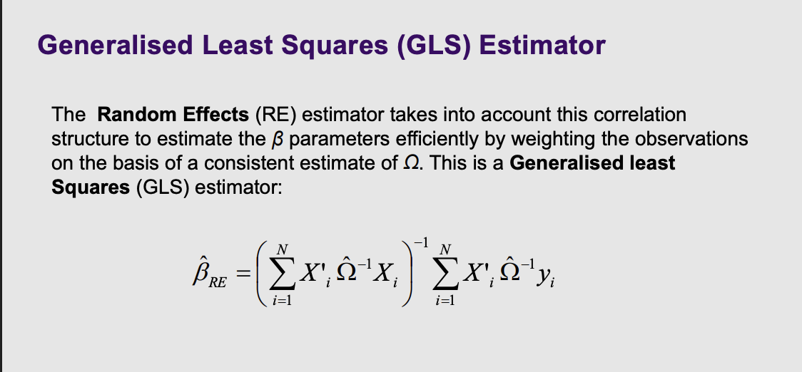
What is the generalised least squares estimator

Generalised Least Squares (GLS) is the mathematical upgrade that fixes this exact problem .

Think of GLS as a smart detective who recognizes when witnesses are just repeating each other.

• Instead of treating all data points equally, the GLS estimator looks at that massive correlation matrix ($\Omega$).

• It realizes, "Ah, these 5 data points all came from John. They share the exact same underlying 'DNA' ($\alpha_i$). Therefore, I shouldn't count them as 5 completely independent pieces of evidence."

• The GLS formula then mathematically weights the observations. It basically downgrades the mathematical importance of redundant data points from the same person, and upgrades data points that bring truly new, independent information.

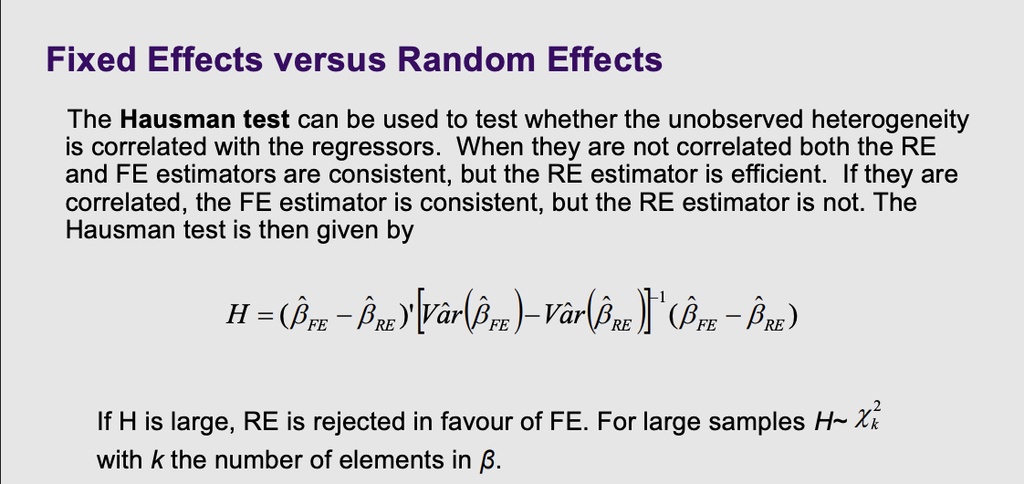
What test can be used to determine whether to use fix or random effects

• What it is: How do you know if you should use Fixed Effects or Random Effects? You ask the referee: The Hausman test.

• How it works: The computer runs both models and compares the answers.

  • If the hidden quirks are not correlated with your data, both models will give you roughly the same answer (but RE is preferred because it's more efficient).

  • If the hidden quirks are secretly contaminating your data, the RE model will fail, and the two answers will look drastically different. If the difference ($H$) is large, you reject Random Effects and are forced to use Fixed Effects .

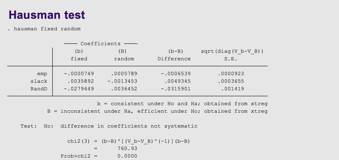
On a stata output what do we look for on the hausman test

• The code hausman fixed random asks the computer to compare the two outputs.

• The Result: Look at the bottom of the slide. Prob>chi2 = 0.0000 . Because this p-value is practically zero, it means there is a massive, systematic difference between the two models .

• The Final Decision: The unobserved hidden traits of these firms are heavily contaminating the data. Random Effects is rejected. The researcher must trust the Fixed Effects model to get the true answer.

• Formal test for endogeneity. Takes the coefficient and compares the different

  H0 is no correlation

   

  P value is the bottom value, smaller than 0.05 and reject the null, there is correlation and just focus on the fixed effects models. Be careful of the unit of measure, if it is a ratio.