Applied Bayesian
1/62
There's no tags or description
Looks like no tags are added yet.
Name | Mastery | Learn | Test | Matching | Spaced | Call with Kai |
|---|
No analytics yet
Send a link to your students to track their progress
63 Terms
What is convergence?
Where the chain has forgotten its initial starting position and is generating samples from the target posterior distribution.
Traceplots should look like a random scatter about a stable value, the Gelman Rubin statistic R^ should be below 1.05.
What is mixing?
Mixing is the rate at which the MCMC sampler explores the target distribution’s parameter space.
Good mixing is where the chain moves rapidly across the space, resulting in low correlation between successive samples.
Poor mixing is where the chain moves slowly, often due to high autocorrelation between samples (e.g. small step sizes in a random walk, or too large step sizes leading to high rejection), leading to a slow exploration of the target distribution
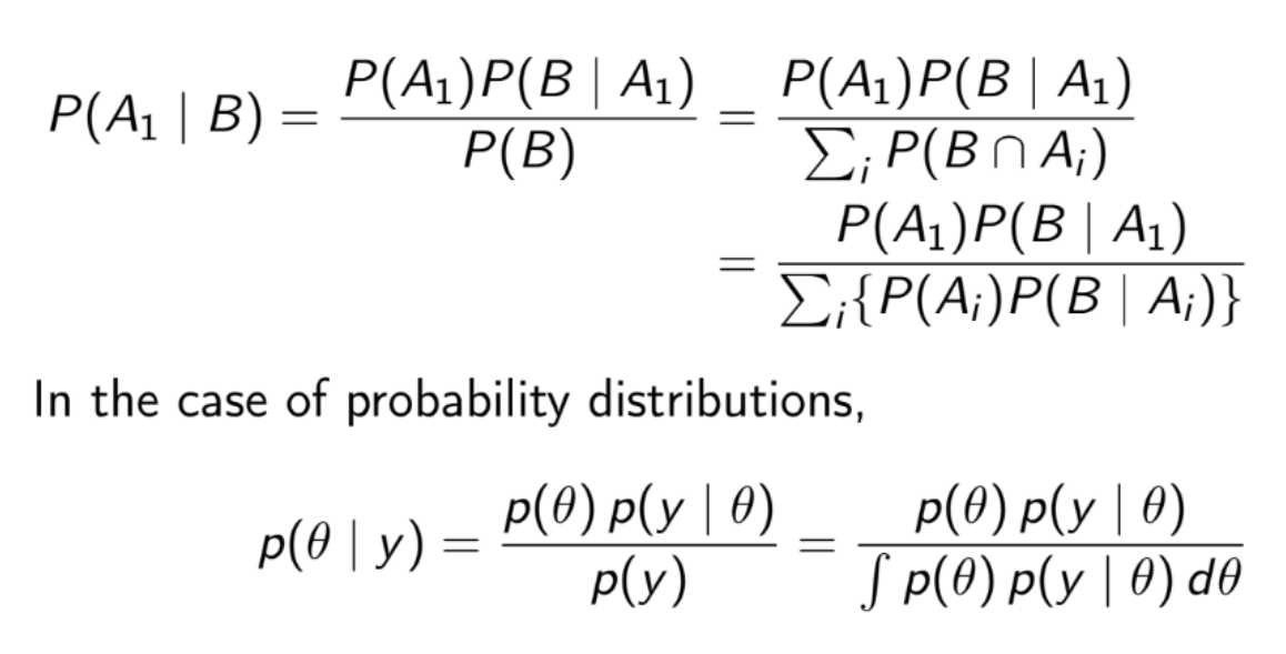
What is the extended form of the Bayes’ theorem?
Use this in practice
P(A∣B)∝P(A)P(B∣A)
P(A’∣B)∝P(A’)P(B∣A)
∴P(A∣B)=P(B∣A)P(A)+P(B∣A′)P(A′)P(B∣A)P(A)
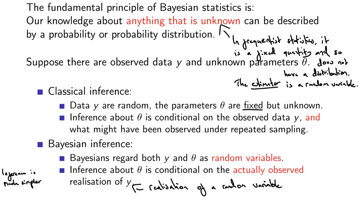
What is the difference between the frequentist and Bayesian interpretations of probability?
The frequentist interpretation is
P[A]=limn→∞nm
where m is the number of times the event A in occurs in a sequence of n independent and identical ‘experiments’
However, this sequence of experiments is hypothetical, and does not actually occur
Frequentist interpretation is based on (potentially) observable events, but we often wish to consider the probabilities of unobservable quantities.
The Bayesian interpretation is that the probability of an event A is a measure of someone’s degree of belief that A will occur.
How do Bayesian and frequentist statistics treat unknown parameters?
What are the mean and variance of a Beta distribution?
m=α+βα
v=(α+β)2(α=β+1)αβ=α+β+1m(1−m)
Useful trick for priors, easier to solve after expressing v in terms of m
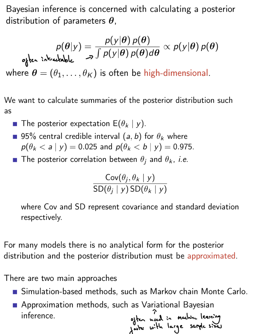
What are Bayesian point estimates?
A point estimate is a numerical summary of the ‘location’ of the posterior distribution
Common choices include the mean, median or mode of the posterior
What is a credible interval?
A set C⊂R is a 100(1−α)% credible interval for θ is
P(θ∈C∣y)=1−α
There are many 100(1−α)% credible intervals
The most widely used is the central credible interval for θ, which is
[θα/2,θ1−α/2]
where θq is the (100×q)th percentile of p(θ∣y), i.e. P(θ≤θq∣y)=q)
We can alternatively use the highest posterior density (HPD) credible interval
C = \{\theta | p(\theta|y) > b \} where b is set such that p(θ∈C∣y)=1−α
The 100(1−α)% HPD interval is the 100(1−α)% credible interval with the shortest width
What is the predictive distribution of Y~, following the same process as observed data y?
p(Y~=y~∣Y=y)=∫p(y~∣θ)p(θ∣y)dθ
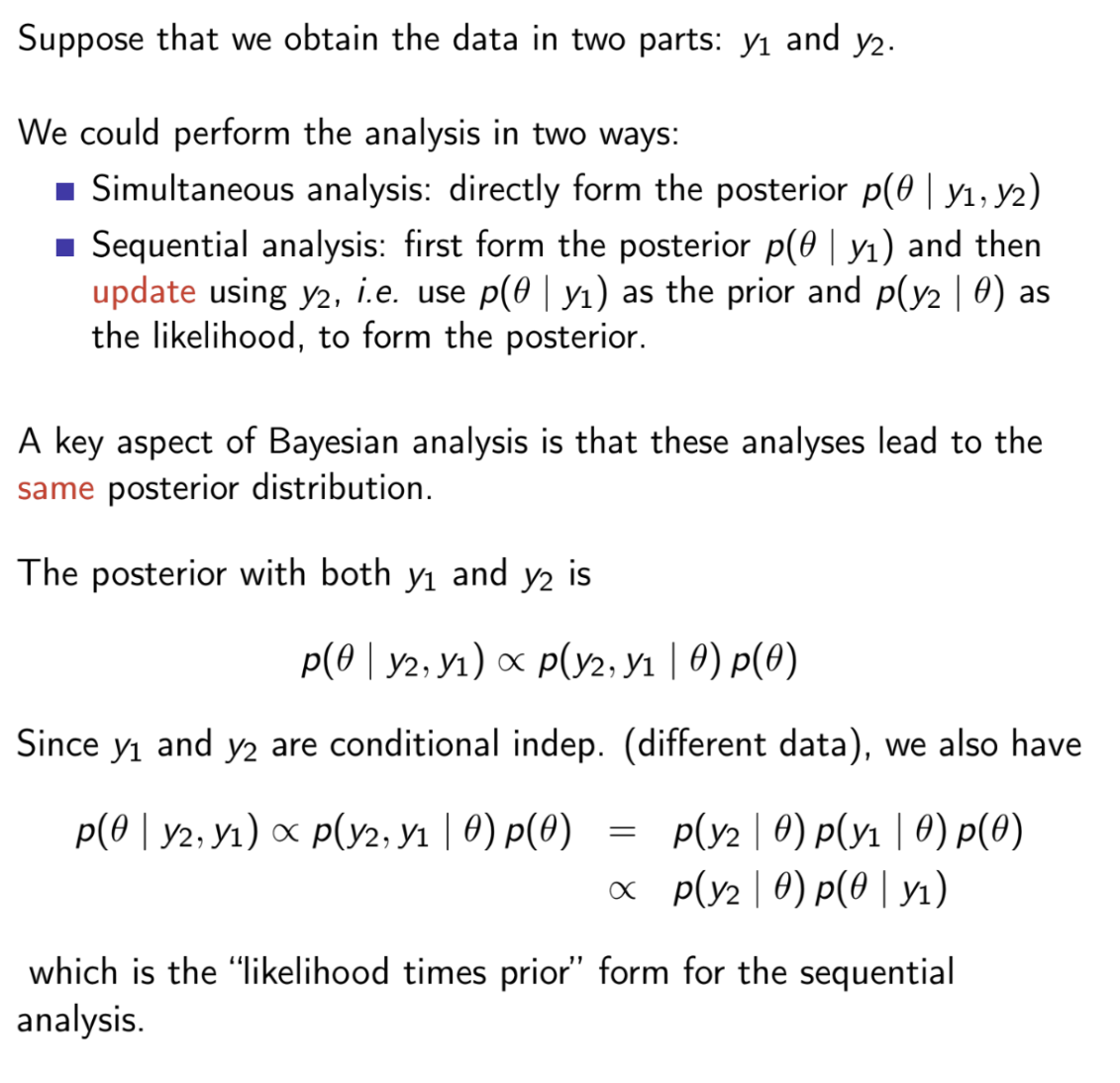
How does sequential analysis work in Bayesian statistics?
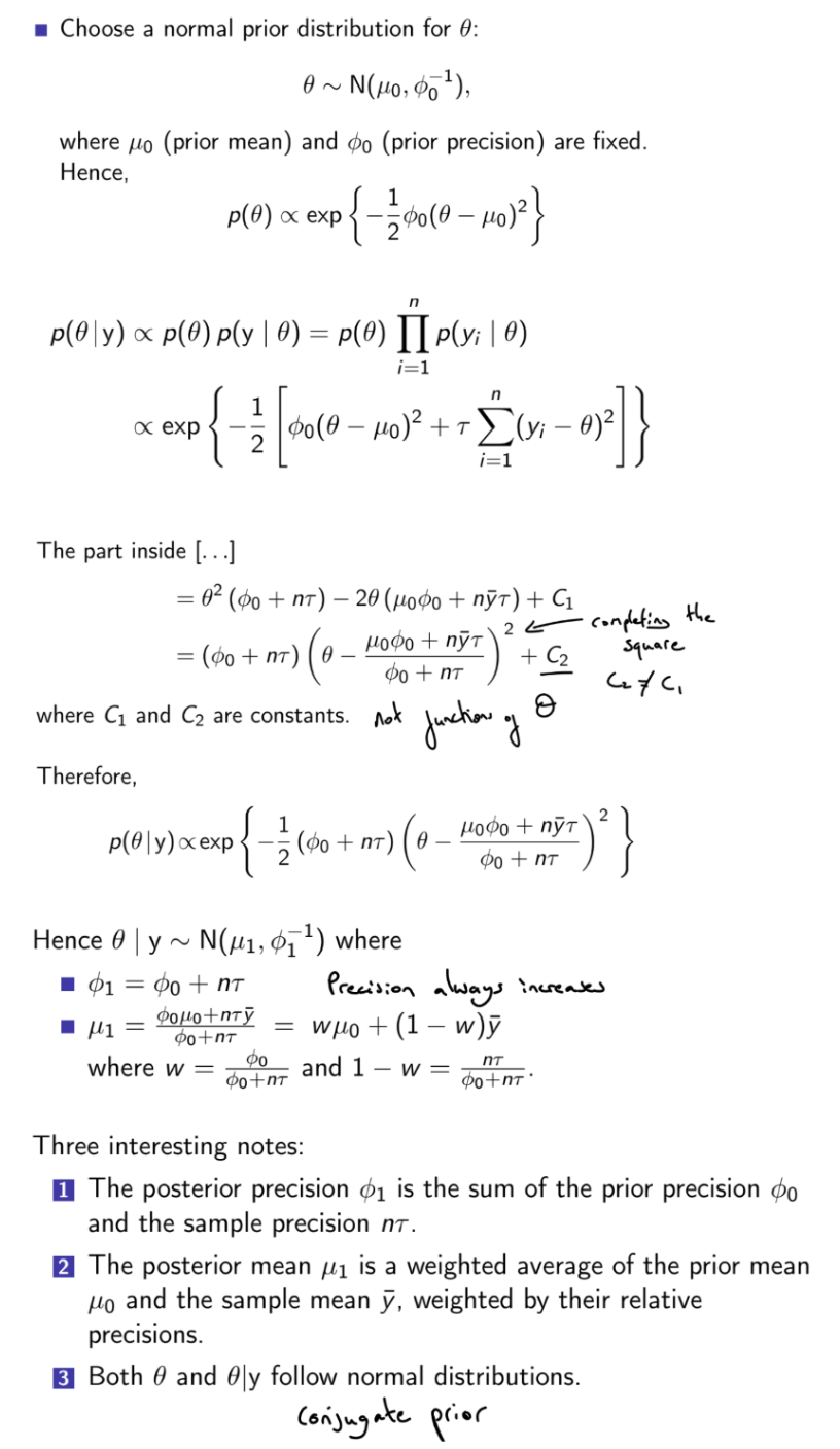
Let Y∣θ∼N(θ,τ−1), where τ is known and θ is unknown and let the prior be θ∼N(μ0,ϕ0−1). How do we obtain the posterior of θ?
If n→∞ with ϕ0 fixed, or ϕ0→0 with n fixed (either lots of data or very diffused prior beliefs) then approximately θ∣y∼N(yˉ,(nτ)−1): the sampling distribution of the MLE.
If we write ϕ0=κ0τ, then
θ∣y∼N(n+κ0nyˉ+n+κ0κ0μ0,((n+κ0)τ)−1)
Hence κ0 may be viewed as a ‘prior sample size’
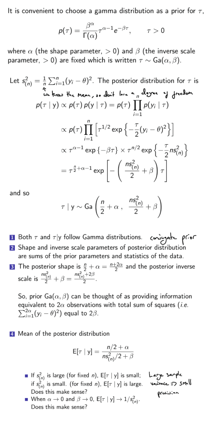
Let Y∣τ∼N(θ,τ−1) , where τ is unknown and θ is known and let the prior be τ∼Gamma(α,β). How do we obtain the posterior of τ?
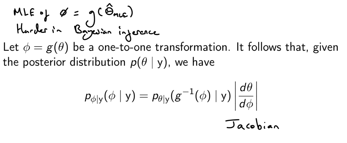
How do we find the posterior distribution of a function of a parameter?
(Rewrite pθ∣y(θ∣y) in terms of ϕ and then multiply by the Jacobin ∣dϕdθ∣
How do we do hypothesis tests in Bayesian statistics?
Choose the hypothesis with the largest posterior probability
Alternatively, can set losses for type I and type II error and calculate expected losses
How can we take into account the support of θ when choosing a prior p(θ)?
For vague priors
For θ∈(−∞,∞) , use θ∼N(0,σ2) where σ2 is very large
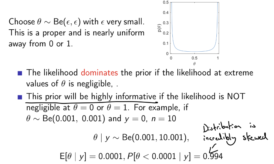
For θ∈(0,∞), use θ∼Gamma(ϵ,ϵ) where ϵ is very small (however, peaked at 0, so highly informative when the likelihood is not negligible near 0)
For θ∈[0,1], use θ∼Beta(ϵ,ϵ) where ϵ is very small (however, peaked at 0 and 1, so highly informative when the likelihood is not negligible near 0 or 1)
![<p><u>For vague priors</u></p><p>For $$\theta \in (-\infty, \infty)$$ , use $$\theta \sim N(0, \sigma²)$$ where $$\sigma²$$ is very large</p><p>For $$\theta \in (0, \infty)$$, use $$\theta \sim Gamma(\epsilon, \epsilon)$$ where $$\epsilon$$ is very small (however, peaked at 0, so highly informative when the likelihood is not negligible near 0)</p><p>For $$\theta \in [0,1]$$, use $$\theta \sim Beta(\epsilon, \epsilon)$$ where $$\epsilon$$ is very small (however, peaked at 0 and 1, so highly informative when the likelihood is not negligible near 0 or 1)</p>](https://assets.knowt.com/user-attachments/1b3b9a35-ca83-4ef7-bf53-79c8a92d462c.png)
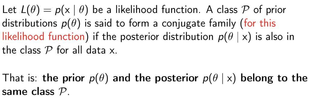
What is a conjugate prior?
A prior is a conjugate prior for a likelihood function p(x∣θ) if the prior p(θ) is in the same family of distributions as the posterior p(θ∣x)
What is a natural conjugate prior?
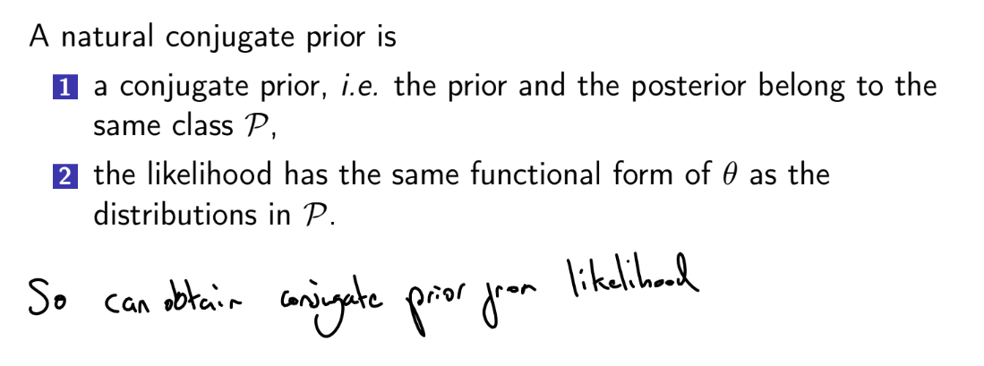
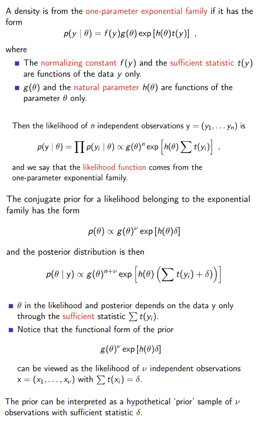
What is the relationship between exponential families of distributions and conjugate priors?
Can use this to find conjugate priors
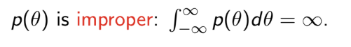
What is an improper prior?
Improper priors are used in Bayesian inference, but can only be used if the posterior will be proper for all possible observable data
What are non-informative priors?
Priors that will be dominated by the likelihood, such that the posterior depends on the data as much as possible. Do not depend on previously obtained information.
e.g. uniform priors (which may be improper), vague / diffused priors (priors with very high variance; p(θ) does not change much over the values of θ for which the likelihood is non-negligible) or Jeffreys’ prior
How does Haldane’s prior differ from the uniform prior?
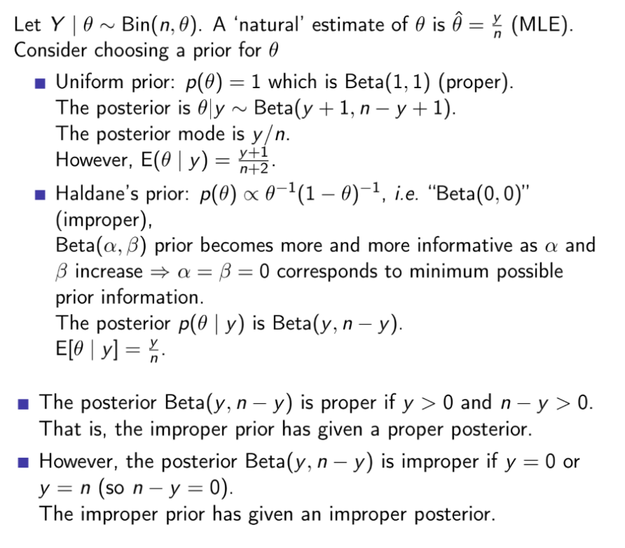
What is the “vague” proper prior for values between 0 and 1?
Are uniform priors invariant to transformations?
No.
A prior for a parameter θ, p(θ), implies that the prior distribution of ϕ=g(θ) is
pΦ(ϕ)=pΘ(θ)∣dϕdθ∣
For a uniform prior, p(θ)∝1, so pΦ(ϕ)∝∣dϕdθ∣. This is constant only if ∣dϕdθ∣ is constant, i.e. g() is a linear transformation
Therefore we can’t have uniform priors for both θ and a non-linear transformation g(θ)
What is Jeffreys’ prior?
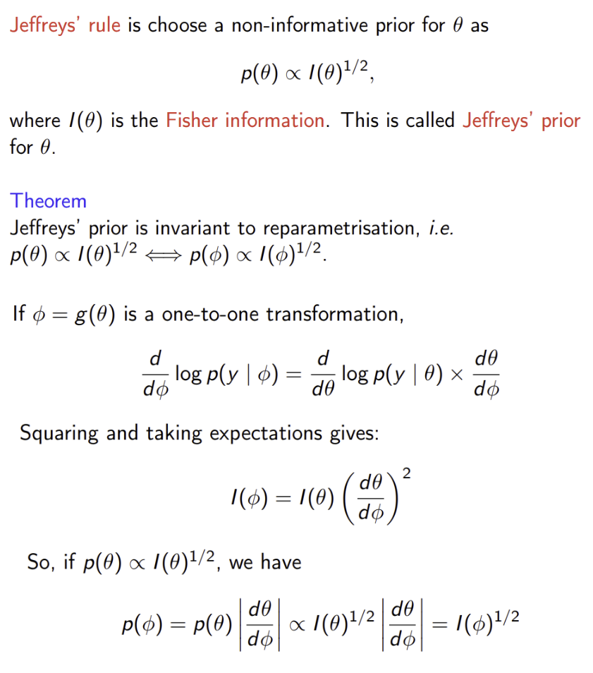
If we know the distribution of θ, what is the distribution of ϕ=g(θ)?
fΦ(ϕ)=fΘ(θ)∣dϕdθ∣=fΘ(g−1(ϕ))∣dϕdθ∣
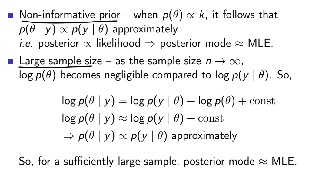
When is the posterior mode approximately equal to the MLE?
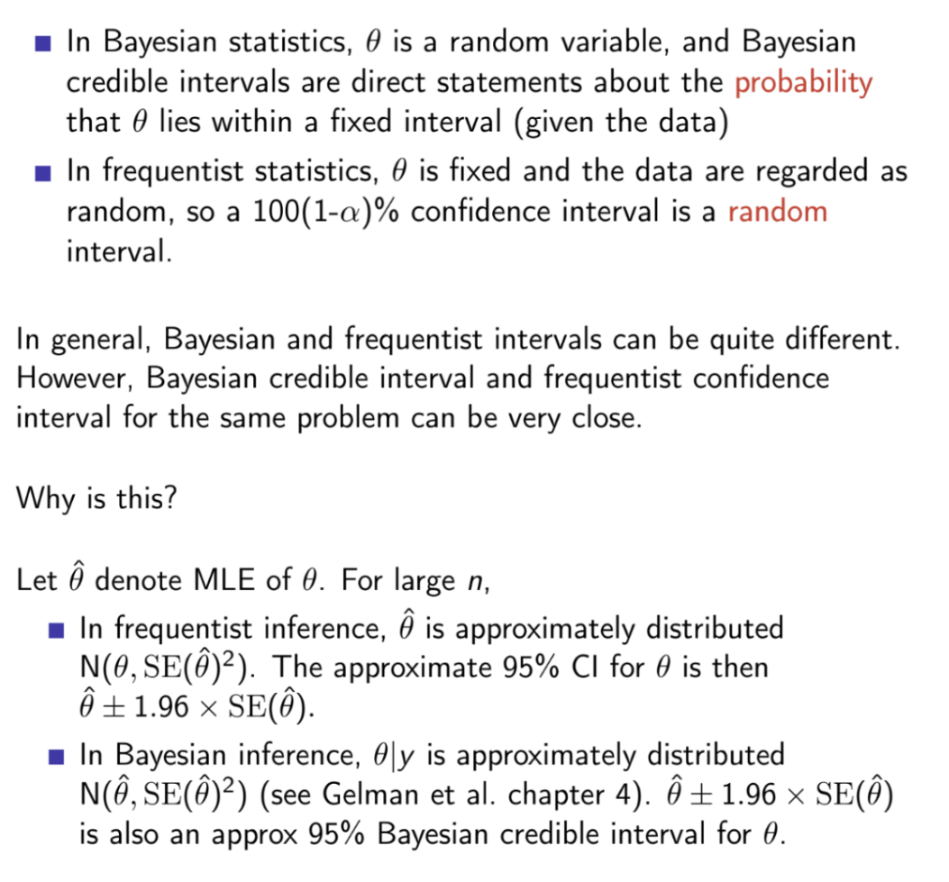
What is the difference between credible intervals and confidence intervals?
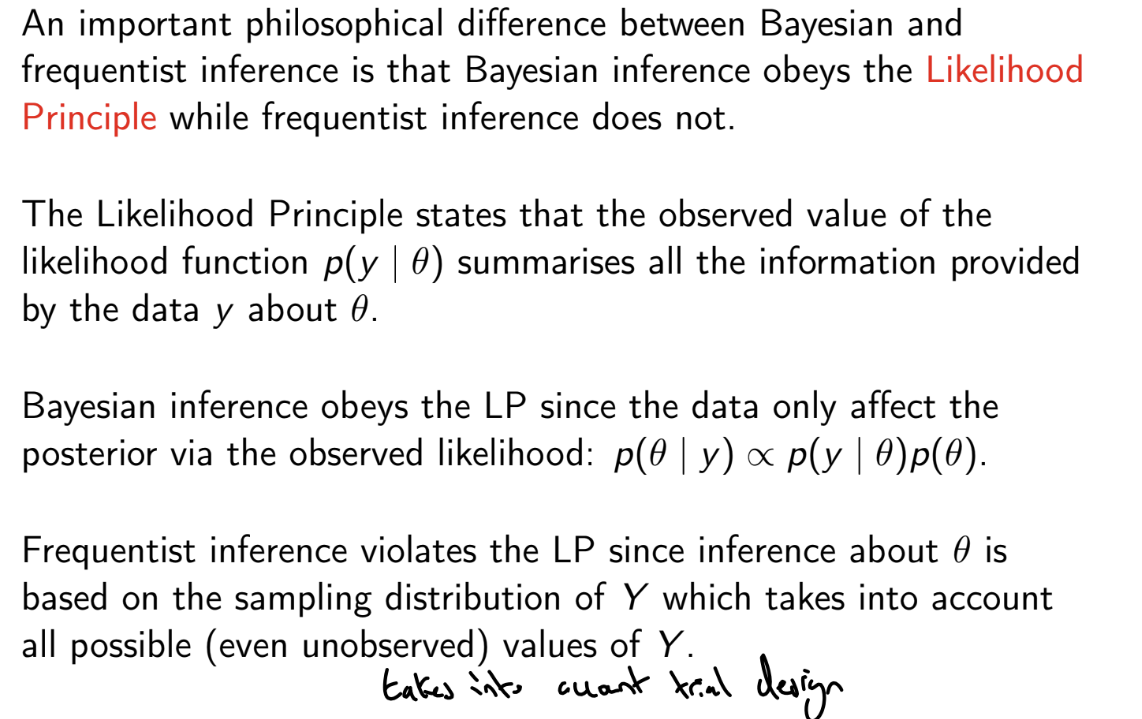
What is the Likelihood principle?
The LP implies that it matters only what was observed, and not what might have been observed. However, the frequentist approach depends not only on what was observed, but also on the design of the study (e.g. how the experiment was stopped, binomial and negative binomial likelihoods differ)
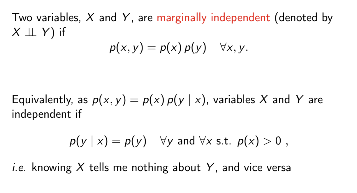
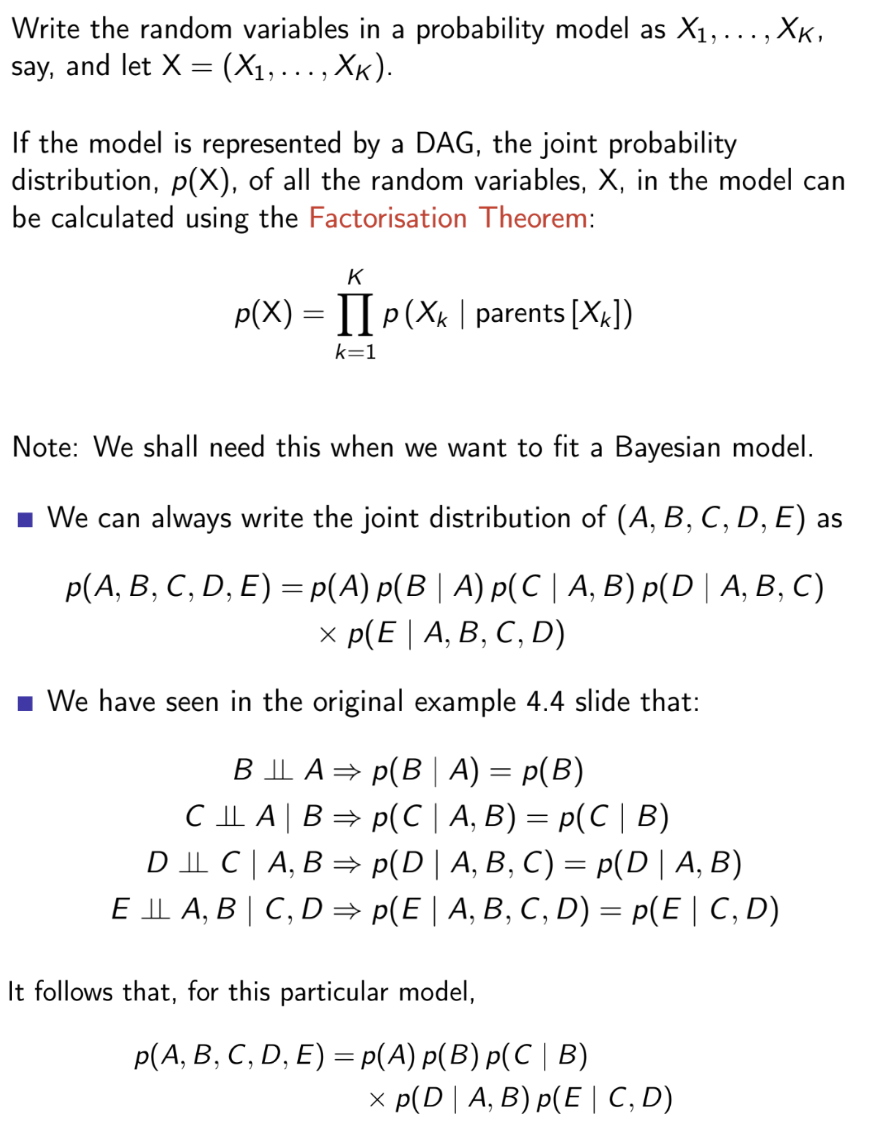
What is marginal independence?
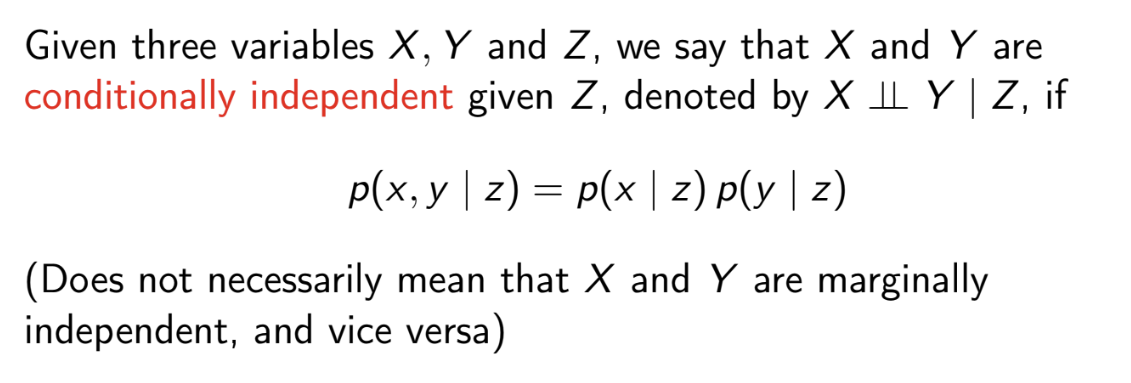
What is conditional independence?
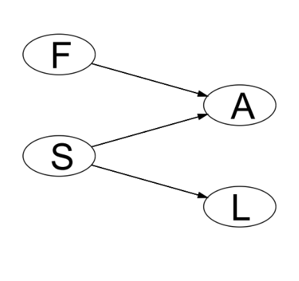
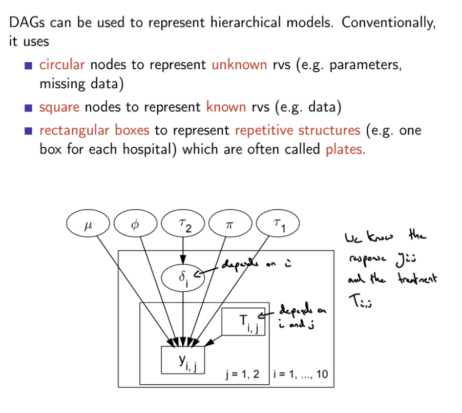
What is a DAG?
A Directed Acyclic Graph is a directed graph (all nodes are random variables, all edges are arrows) that contains no directed cycles
A directed edge / arrow from one node to another indicates that the first variable causes / influences the second. Dashed arrows denote deterministic dependencies, solid arrows denote stochastic dependencies.
DAGs are useful for visualising and investigating conditional dependence, e.g. causal relationships between random variable, where X causes / influences Y, but Y does not cause / influence X
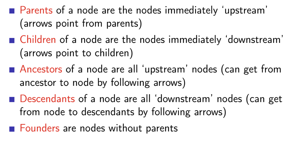
What are parents, children, ancestors, descendants and founders in DAGs?
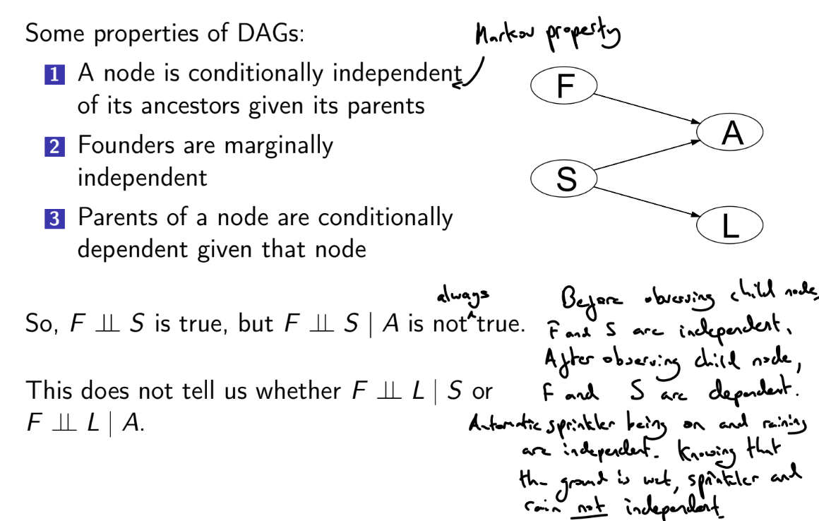
What are the dependence properties of DAGs?
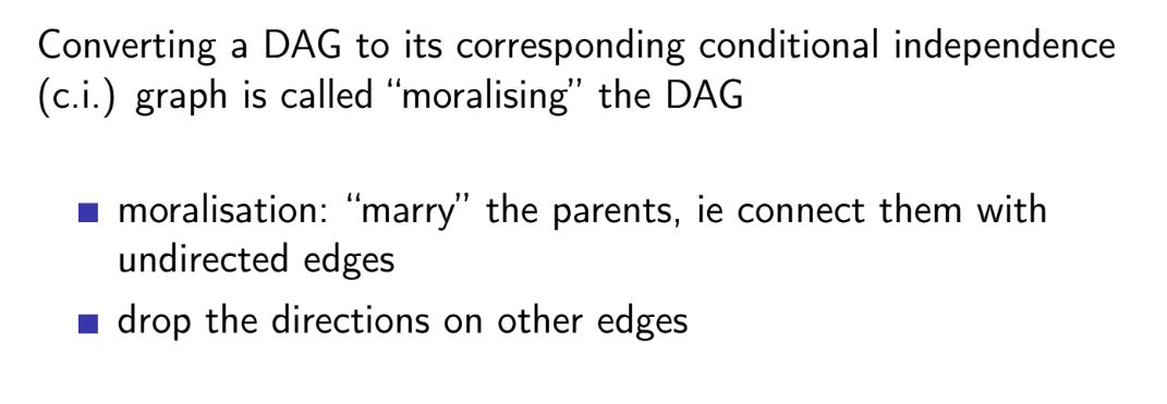
What is moralising a DAG?
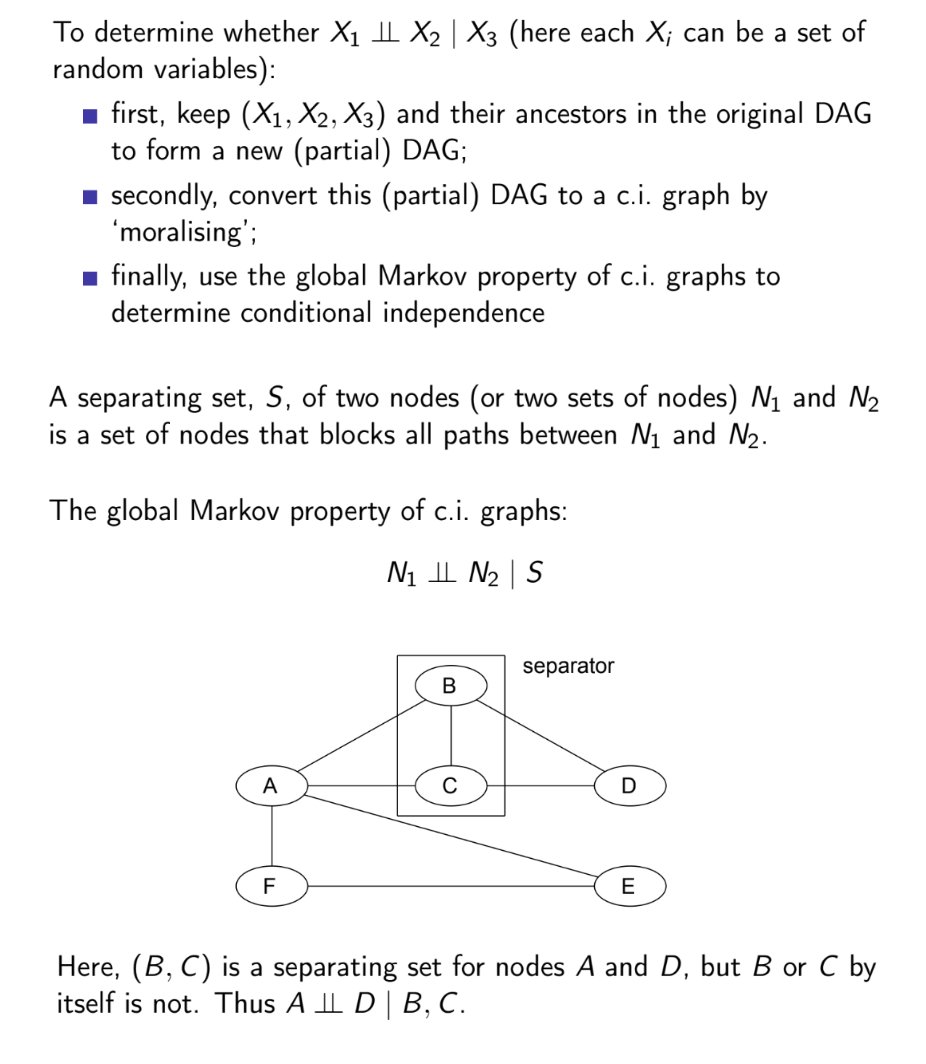
How can we use DAGs to determine whether variables are conditionally independent?
c.i graph = conditional independence graph
only draw relevant variables and their ancestors in the partial DAG
What is the factorisation theorem?
Proceeds from the fact that a variable is conditionally independent of its ancestors given its parents
What is a Markov Blanket?
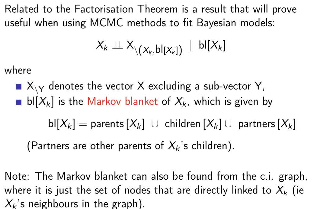
What is the full-conditional distribution of Xk?
P(Xk∣X\Xk)∝P(X)=∏i=1KP(Xi∣parents[Xi]) (factorisation theorem)
P(Xi∣parents[Xi] is constant with regards to Xk if Xk is neither Xi or a parent of Xi
So P(Xk∣X\Xk)∝P(Xk∣parents[Xk])∏w∈children[Xk]P(w∣parents[w])
![<p>$$P\left(X_{k}|X_{\backslash X_{k}}\right)\propto P(X)=\prod_{i=1}^{K}P(X_{i}|\text{parents}[X_{i}])$$ (factorisation theorem)</p><p>$$P(X_{i}|\text{parents}[X_{i}]$$ is constant with regards to $$X_k$$ if $$X_k$$ is neither $$X_i$$ or a parent of $$X_i$$</p><p>So $$P(X_k | X_{\backslash X_k}) \propto P(X_k | \text{parents}[X_k]) \prod_{w\in children[X_k]} P(w|\text{parents}[w])$$ </p><p></p>](https://assets.knowt.com/user-attachments/5ecb7998-f175-4c4b-a0b8-069bd296059c.png)
What is the motivation for MCMC?
What is a Markov chain?
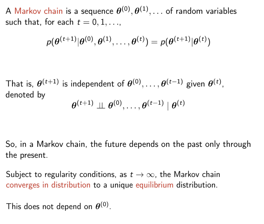
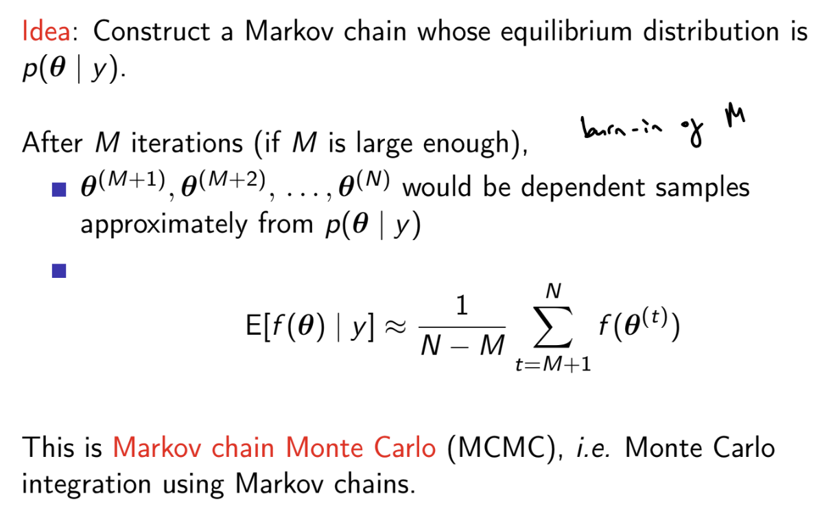
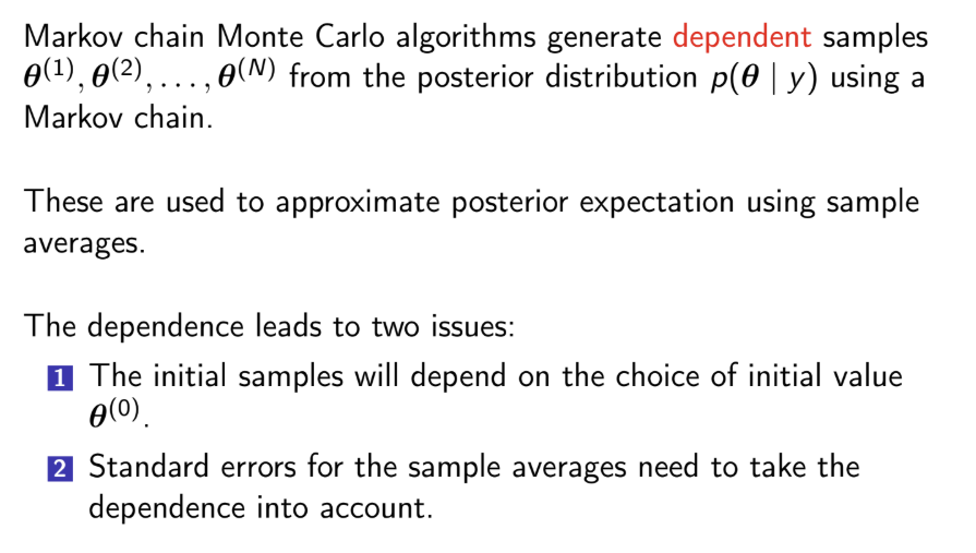
What is MCMC?
For any function of the parameters, simply calculate f(i)=f(θ(i) to obtain a sample from its posterior distribution. Can then calculate posterior mean / median / mode, etc.
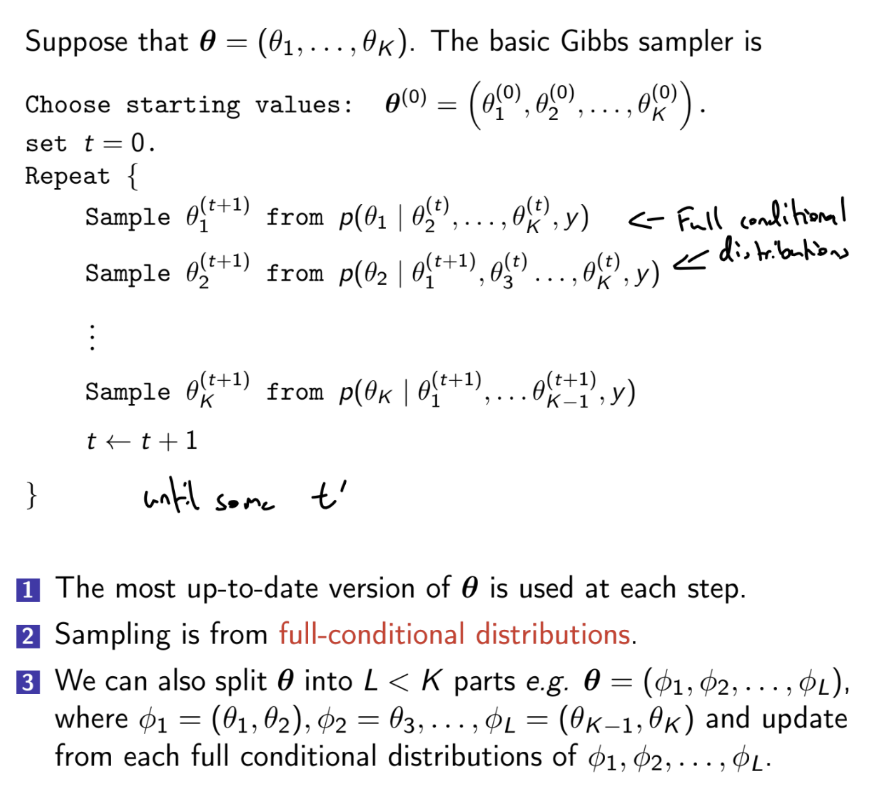
What is the Gibbs sampler algorithm?
The full conditional distribution of a parameter may be a known distribution, which can be sampled from simply
If the full conditional distribution is not proportional to a kernel of a known distribution, the full conditional distribution would need to be sampled using a method such as the Metropolis-Hastings algorithm (Metropolis within Gibbs) or rejection sampling
What are the two ways of obtaining the full-conditional distribution for a variable?
P(C∣V\C)∝ terms in joint distribution containing C
Factorisation theorem - Joint distribution P(V)=∏v∈VP(v∣parents[v])
P(C∣\V)∝P(C∣parents[C])w∈children[C]∏P(w∣parents[w])
How can we use DAGs to represent hierarchical models?
What are the issues that arise due to dependence between MCMC samples?
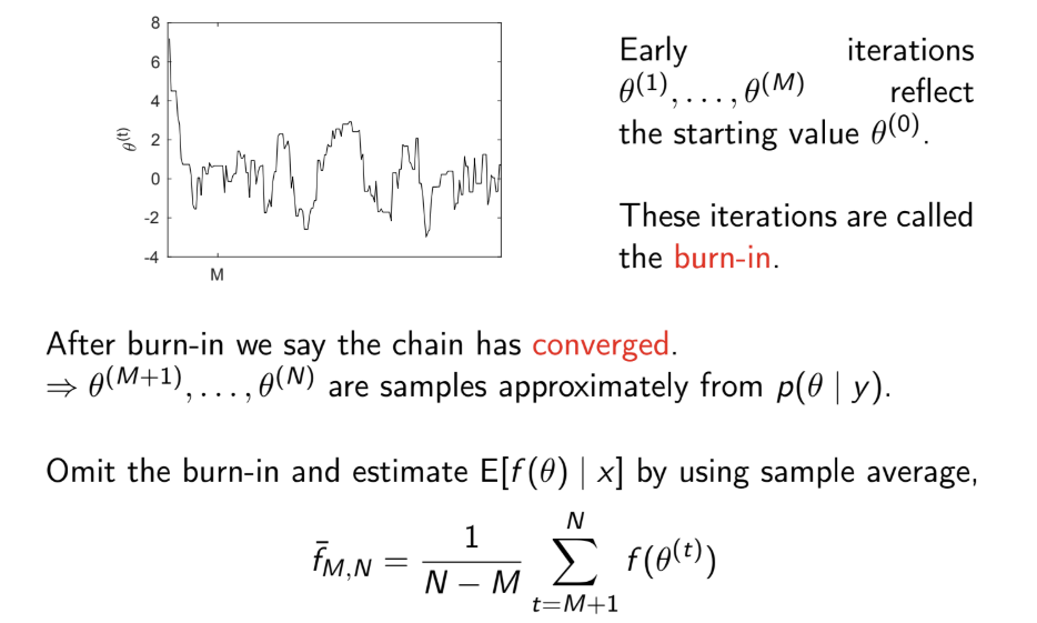
What is burn-in?
The burn-in are the first M samples of the chain, which are discarded because it is believed that the chain has not yet converged and that these values are still dependent on the initial values.
Strictly speaking, convergence is only achieved for M=∞
In practice, we can only detect lack of convergence
If no evidence of lack of convergence is found, we are more confident that the chain has converged
We can check this:
using traceplots: once convergence has been reached, samples should look like a random scatter about a stable value
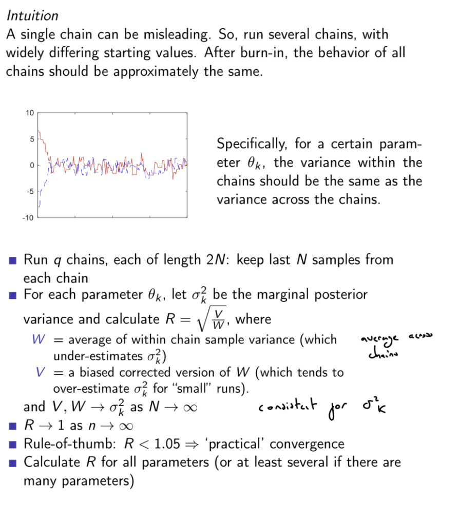
using convergence diagnostics: if the Gelman-Rubin diagnostic \hat{R} < 1.05, this indicates practical convergence
Use these to set M, the length of the burn-in
What is the Gelman-Rubin statistic?
Compares within chain and between chain variation
How can we determine how long to run MCMC chains for?

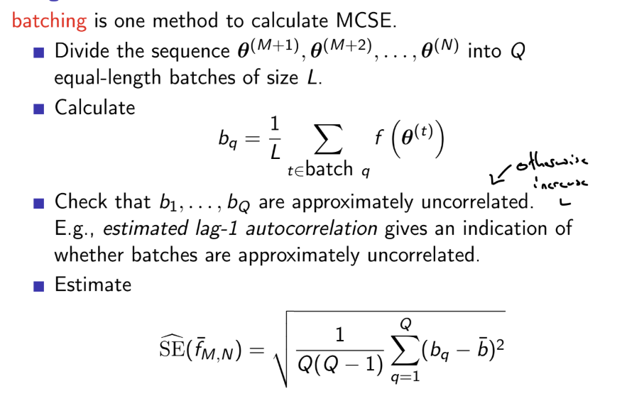
What are batch mean SEs?
Divide by Q(Q-1) because we are estimating the variance of b^, not an individual b
Can also account for auto correlation via time series SEs
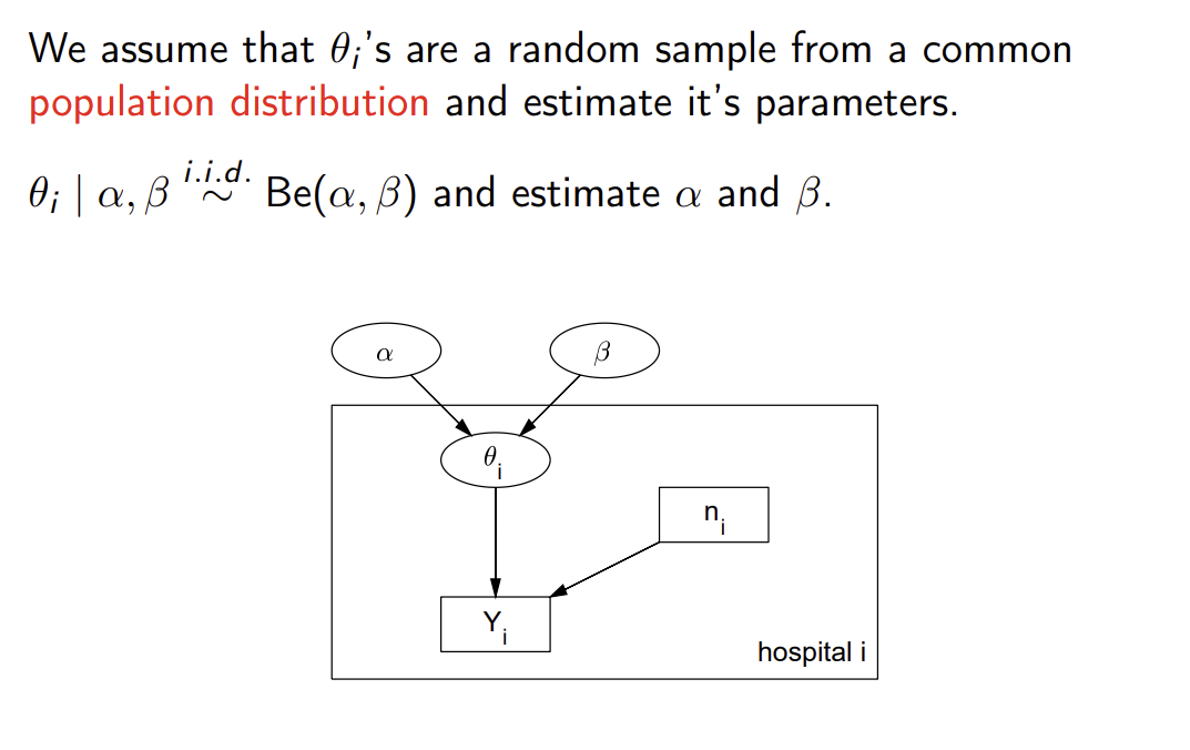
What are Bayesian hierarchical models?
Also called random effect or multi-level models
We assume that the parameters θ of groups are a random sample from a common population distribution, and then estimate the (hyper-)parameters of that population distribution
We assign a (hierarchical) prior distribution to the hyper-parameters.
We have:
Likelihood p(y∣θ) (1st level)
Prior p(θ∣ϕ2) with higher level parameter ϕ2 (2nd level)
Prior p(ϕ2) (3rd level)
We can add further levels, with ϕk being k-th level hyper-parameters. A non informative prior is usually specified for the top level parameters.
These models imply that θi is different for every group, but similar - θi are not marginally independent, but are exchangeable
By assuming that the parameters are drawn from a common population distribution, the more extreme parameters are shrunk towards the overall mean. The posterior distribution for each θi borrows strength from the likelihood contributions of all groups, via their influence on the unknown population parameters, and reflects our full uncertainty about the true values of the population parameters. These models are also useful if we are interested in the population parameters themselves.
Better than assuming a common θ between all groups, or that the parameters θi for each group are independent (we want to use information about θ\i to estimate θi)
Can obtain full conditional distribution for each parameter and then use Gibbs sampler
What is exchangeability and the general representation theorem?
A sequence of random variables θ1,…,θn is exchangeable if, for any permutation {i1,…,in} of {1,…,n}, (θi1,…,θin) has the same n-dimensional joint probability distribution as (θ1,…,θn)
i.e. for all a1,…,an,
p(θ1=a1,…,θn=an)=p(θi1=a1,…,θin=an)
If θ1,…,θn are marginally independent and have the same marginal distribution (they are i.i.d), then they are exchangeable
The General representation theorem shows that if θ1,…,θn are exchangeable, there there exists a parametric model p(θ∣ϕ) with prior p(ϕ) for ϕ such that θi⊥⊥θj∣ϕ and therefore θi∣ϕ∼iidp(θ∣ϕ)
Exchangeability therefore implies a hierarchical model: this is equivalent to θ1,…,θn being a random sample from a model p(θ∣ϕ) with prior p(ϕ)
When is it reasonable to assume exchangeability?
The parameters of groups, θ1,…,θn, are exchangeable if, for any permutation {i1,…,in} of {1,…,n}, (θi1,…,θin) has the same n-dimensional joint probability distribution as (θ1,…,θn): e.g. there is no reason to believe that θi=a and θj=b is more likely than θi=b and θj=a
However, if we know additional information about the groups, exchangeability may not be a reasonable assumption; we may have reason to expect one group’s parameter to be greater than another’s.
Whether it is reasonable to assume exchangeability depends on our degree of knowledge / ignorance.
We can address this by including covariates in our hierarchical models, e.g. a generalised linear mixed model
What is the Metropolis-Hastings sampler?
The Metropolis-Hastings sampler produces a chain of values θ(1),θ(2),… from a distribution with density g(θ) (e.g. full conditional or posterior)
Choose θ(0) then, at the i-th iteration
Propose θ’ from a proposal distribution q(θ(i−1),θ’)
(Via a simulated uniform random variable) Accept this proposal with probability α(θ(i−1),θ’)=min{1,g(θ(i−1)q(θ(i−1),θ‘)g(θ’)q(θ‘,θ(i−1))}
There are two main types of proposal distribution:
The random walk sampler, where θ’=θ(i−1)+ϵi where the distribution of ϵi is zero-mean and symmetric (e.g. normal, t-distribution)
Then q(θ(i−1),θ’)=q(θ‘,θ(i−1)): always accept uphill moves, sometimes accept downhill moves
The variance of ϵi is a tuning parameter. Too low step-size will lead to suggestions of small deviations and a high acceptance rate, causing random walk behaviour and poor mixing (explores sample space slowly). Too large step-size will lead to suggestions of large deviations and a low acceptance rate, causing a ‘sticky’ chain with high autocorrelation and poor mixing. High autocorrelation in the chain will result in a high variance of estimators.
The independence sampler, where the proposal distribution does not depend on the previous state θ(i−1), i.e. q(θ(i−1),θ’)=q(θ’)
This method works well when q(θ) is a good approximation of g(θ). Can move from 1 side of the distribution to another, better mixing than random walk. However, if it is a poor approximation, we will reject most proposals, leading to a sticky chain
How do we tune Metropolis Hastings random walk samplers?
The random walk sampler is θ’=θ(i−1)+ϵi where the distribution of ϵi is zero-mean and symmetric (e.g. normal, t-distribution)
Then q(θ(i−1),θ’)=q(θ‘,θ(i−1)): always accept uphill moves, sometimes accept downhill moves
The variance of ϵi is a tuning parameter. Too low step-size will lead to suggestions of small deviations and a high acceptance rate, causing random walk behaviour and poor mixing (explores sample space slowly). Too large step-size will lead to suggestions of large deviations and a low acceptance rate, causing a ‘sticky’ chain with high autocorrelation and poor mixing.
High autocorrelation in the chain will result in a high variance of estimators.
It can be shown that, in general, samplers will the lowest variability have an average acceptance rate which is between 0.2 and 0.3
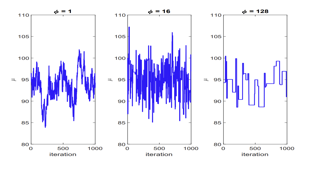
What problems does correlation cause in the Gibbs sampler?
The Gibbs sampler works by sampling from each full conditional distribution. This can lead to slow mixing if the posterior distribution has high correlation between some variables.
e.g. let Var(X1)=Var(X2)=1 and Cov(X1,X2)=ρ
The full conditional distribution of X1 is N(ρX2,1−ρ2) and vice versa
If ρ is large, the conditional variance of X1∣X2, (1−ρ)2) is small relative to the marginal variance 1, which leads to slower convergence
A second problem is that higher correlation between variables will lead to higher dependence between samples. This autocorrelation will cause the variance of estimators to increase.
There are two main remedies:
Thinning - only take every kth value of the chain, leading to reduced autocorrelation between samples
Reparameterisation - transform from X to some variables with lower correlation
e.g. in the model yi∼Poisson(μi)
and μi=α+βXi
α and β are highly correlated. If we centre X and instead specify μi=α+β(Xi−Xˉ) , then this removes the correlation between α and β
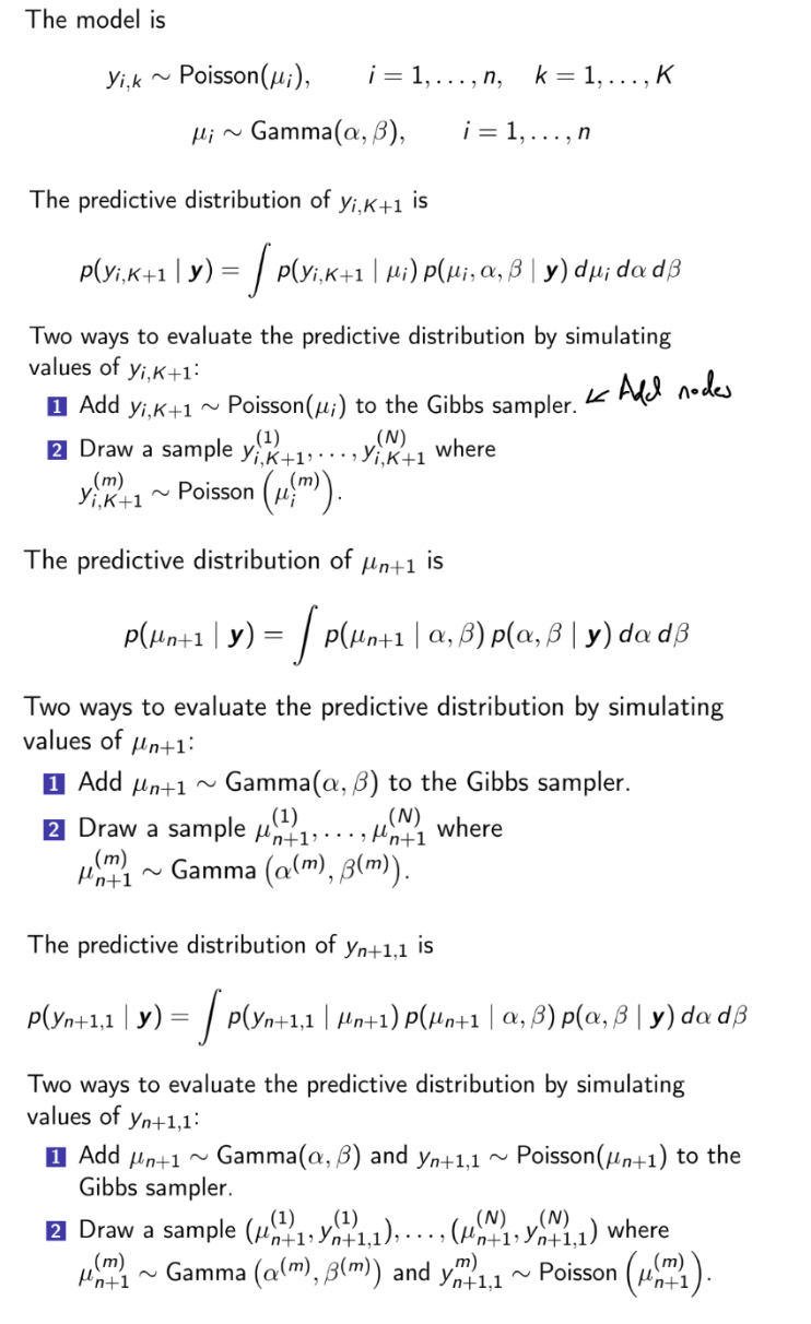
For hierarchical models, what is the predictive distribution of a new value in a group, a parameter for a new group, and a new value in a new group?
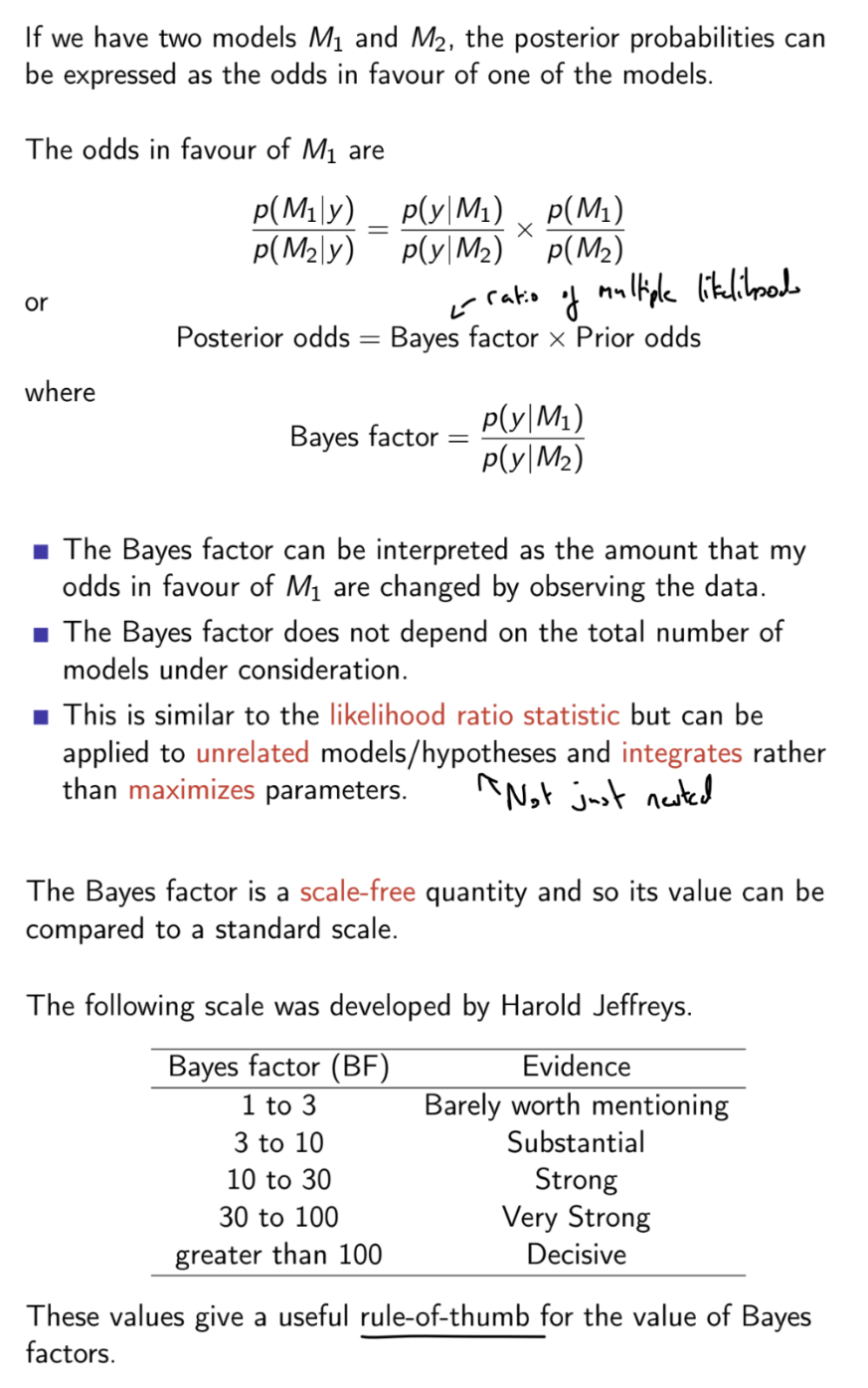
What is the Bayes factor?
Disadvantages: very difficult to work out Bayes factor analytically for more complex models
Lindley’s paradox: if comparing a model M1 where a parameter is set with a model M2 where a parameter is given a prior, we can choose a weight on that prior to make the Bayes factor in favour of M2 arbitrarily small. Bayes factors are sensitive to the choice of the weight on the prior: should choose a sensible prior variance of any parameters.
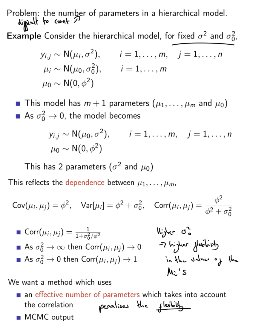
Why can’t we simply use number of parameters in Bayesian hierarchical models?
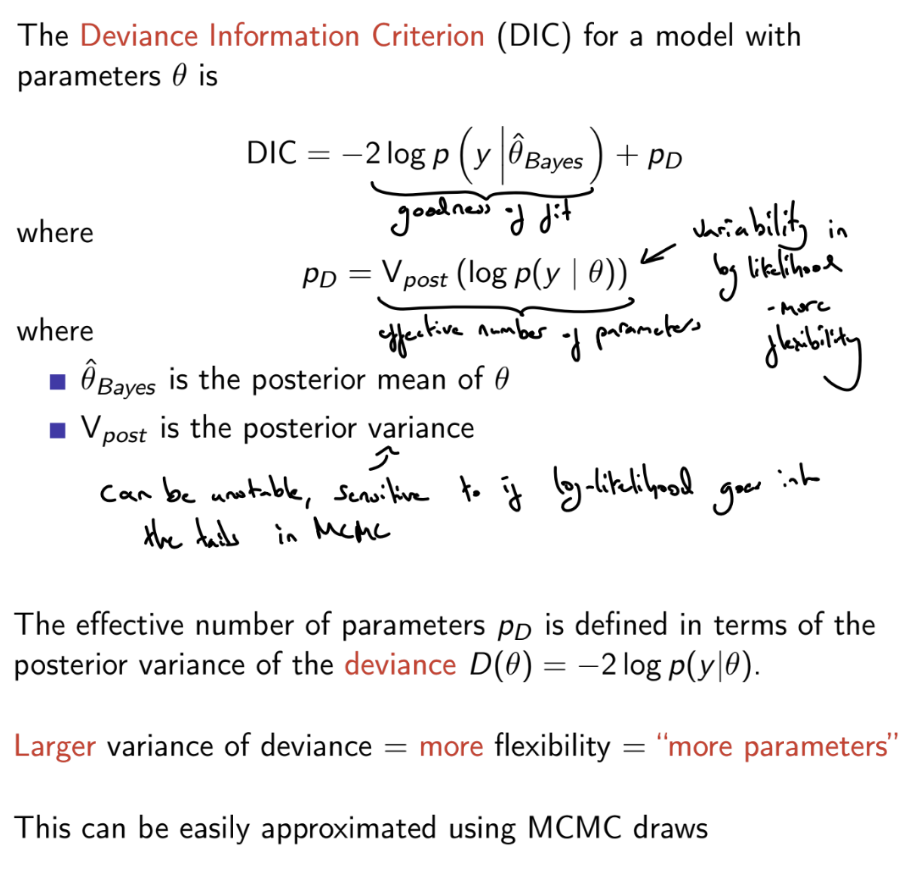
What is the Deviance Information Criterion (DIC)?
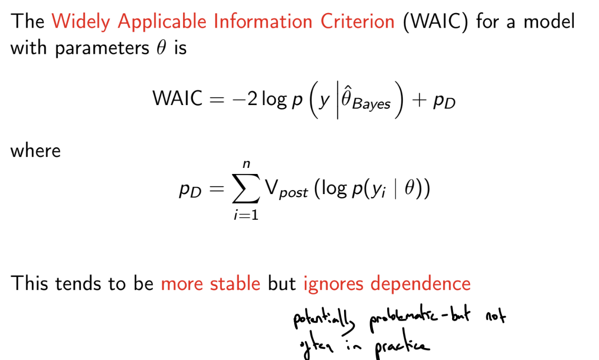
What is the Widely applicable information criterion (WAIC) ?
More stable than the Deviance Information Criterion
How can we carry out cross-validation of Bayesian models?

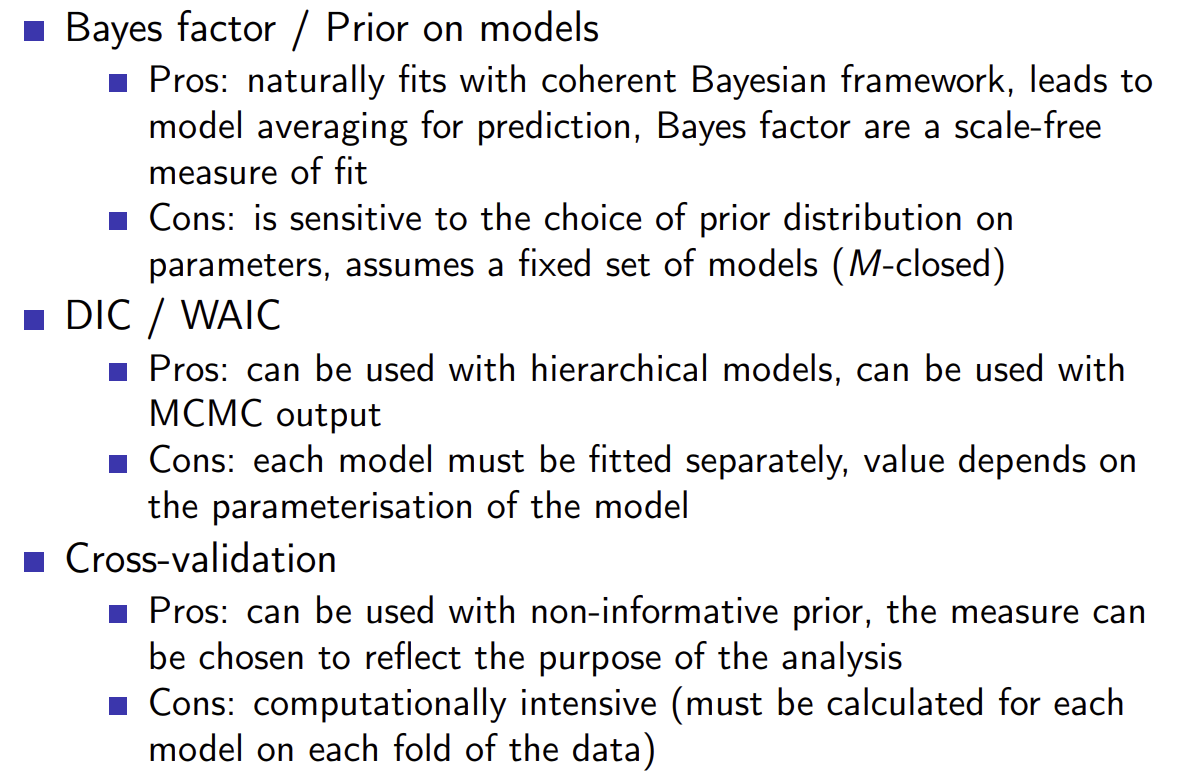
What are the pros and cons of using Bayes factor, DIC / WAIC and cross-validation to evaluate Bayesian models?
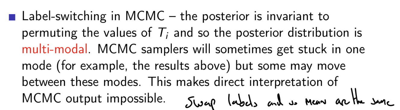
What is the label switching problem in mixture models?