EAE3111 Chapter 6

Mean

Seasonal or daily cycles

Variability

Difference to the long time mean

Standard deviation

Spread of a distribution, strength of the variability

Correlation

How much two variables tend to have anomalies at the same time

Central limit theorum

Tendency of long term averages to have less variation than a single data point

Time scale dependence of variability

Increasing the time scale reduces the variability

Characteristics of climate variability: strength

More variability over land

Characteristics of climate variability: time scales

Longer time scales have less variability, different regions have different time scales.

Oscillation

Positive and negative anomalies taking turns on irregular time intervals

Chaotic

Persistence of anomalies

Trend

The climate drifts on one direction over time

Characteristics of climate variability: spatial scales

Generally larger variability over land, varies between regions.

Teleconnections

Unexpected connections between remote regions

Hoevmoeller diagram

Presents the variability of a climate variable as a function of a spatial direction versus the time dimension

Shorter time scale variability tends to be on

Smaller spatial scales

Longer time scale variability tends to be on

Larger spatial scales

External influences on the climate system

Climate system cannot feedback (changes in insolation, volcanic eruptions, anthropogenic forcing or meteorites)

Internal influences on the climate system

Dynamics of the climate system within itself given external boundary conditions

A stable equilibrium system

A dynamical system which, given initial conditions and certain fixed boundary conditions, would converge towards an equilibrium point.

Oscillating system

Highly predictable repeating cycle, with some internal variability

Deterministic chaos system

Tendency equations of the system are known (deterministic) but the system is largely unpredictable, varying around equilibria points in a non-periodic, chaotic and unpredictable way.

The Lorenz-salzman model

Simplified convection dynamics which illustrate the important characteristics of chaotic weather dynamics.

The Lorenz model has

3 equilibria

Characteristics of the Lorenz-Salzman model: no stable equilibria

Always varies, no valleys in the climate potential POV

Characteristics of the Lorenz-Salzman model: regime behaviour

Oscillations between two non-zero equilibria (attractors) with transitions between two regimes.

Characteristics of the Lorenz-Salzman model: non-periodic flow

The system never reaches the same point twice.

Deterministic

The tendency equations are exactly defined if the state of the system is known.

Chaos

The time evolution beyond a given time interval cannot be predicted, no matter how well the initial state of the system is known.

Characteristics of the Lorenz-Salzman model: chaotic time evolution

Only predictable up to a certain time period, depending on how precisely the initial conditions is known. There will be a point where the system fills all likely points in dynamical space.

Characteristics of the Lorenz-Salzman model: numerical uncertainty

No general analytical solution, thus must be estimated with numerical approximations, which are limited by computer precision.

Characteristics of the Lorenz-Salzman model: non-linear response to forcing

As the distribution shifts, the shape changes (shifting to higher values results in the lower value regime becoming more likely)

Stochastic climate variability

Randomness of climate variability on larger and longer time and spatial scales results from chaotic weather on shorter and smaller time and spatial scales.

The Power Spectrum

How much each frequency contributes to the variability of the time series

Area under the power spectrum curve

Total variance over the range of frequencies

White noise

Power spectrum has the same amount of variance for all frequencies, result of a time series of purely random numbers.

Red noise

Climate can vary on long time scales without a cause (external forcing) simply due to the weather variability that exist on shorter time scales.

Red Noise Null Hypothesis

The system is linearly damped and forced by white noise (random weather)

Slab ocean model

An example of red noise process, the ocean is just a heat capacity that integrates atmospheric sensible heat fluxes

Glacier red noise model

An example of a red noise process, the glaciers mass is controlled by random weather events of snow accumulation and melting

SST variability is in the order of

0.5ºC

Elements of the spatial complexity: domain boundaries

Coastlines or mountains

Elements of the spatial complexity: different mean states

Wind directions, temperature

Elements of the spatial complexity: different dynamics

Coriolis force or water vapour saturation pressure

Principle component analysis or empirical orthogonal functions (EOFs)

Dimensionality reduction to explain the maximum amount of variance in data.

Statistical modes

Has three elements: Data = Amplitude * EOF Pattern * time series

Climate variability of the domain at any given time

Sum of all modes with the pattern * the amplitude * the current value of the time series

Mode hierarchy

The modes are in order by how much of the data they can explain

Maximum variance

The EOF analysis is the optimal approach to maximise the explained variance in one mode

Orthogonal

The EOF modes are not similar to each other, thus the time series and patterns of two modes is uncorrelated

Multipoles

Orthogonality constraints lead to multi-pole like patterns in the whole domain.

Null hypothesis for spatial structure

Nearby regions will influence each other to behave similarly over time (isotropic diffusion), red noise but on the spatial scale

Climate mode

A reappearing pattern in space or time that is potentially predictable beyong stochastic red noise.

Deviation from chaos

Structure in variability beyond the simple stochastic model

A phyiscal mode

You can predict the next phase of the oscillator by knowing the current state of the system, a swing or a pendulum

Phase space

The system moves from one phase to the next in a highly predictable manner

Two variables can be measured with an out-of-phase relation

Position and velocity

When position is at maximum

Velocity is at zero

Level 1: subjective / impact focused

Usually defined based on a statistical mode, subjective, no physical oscillator or deviations from pure noise.

Damped persistence

Current anomalies will persist in the near term, but mathematically decay toward zero

Level 2: structures different from noise

Indications of deviations from pure noise, not clear is this is a physical mode, could be chaotic but different from red noise.

Level 3: a physical mode/predictable oscillator

A structure different from red noise, physical phase space with clear propagation, predictable beyond damped persistence

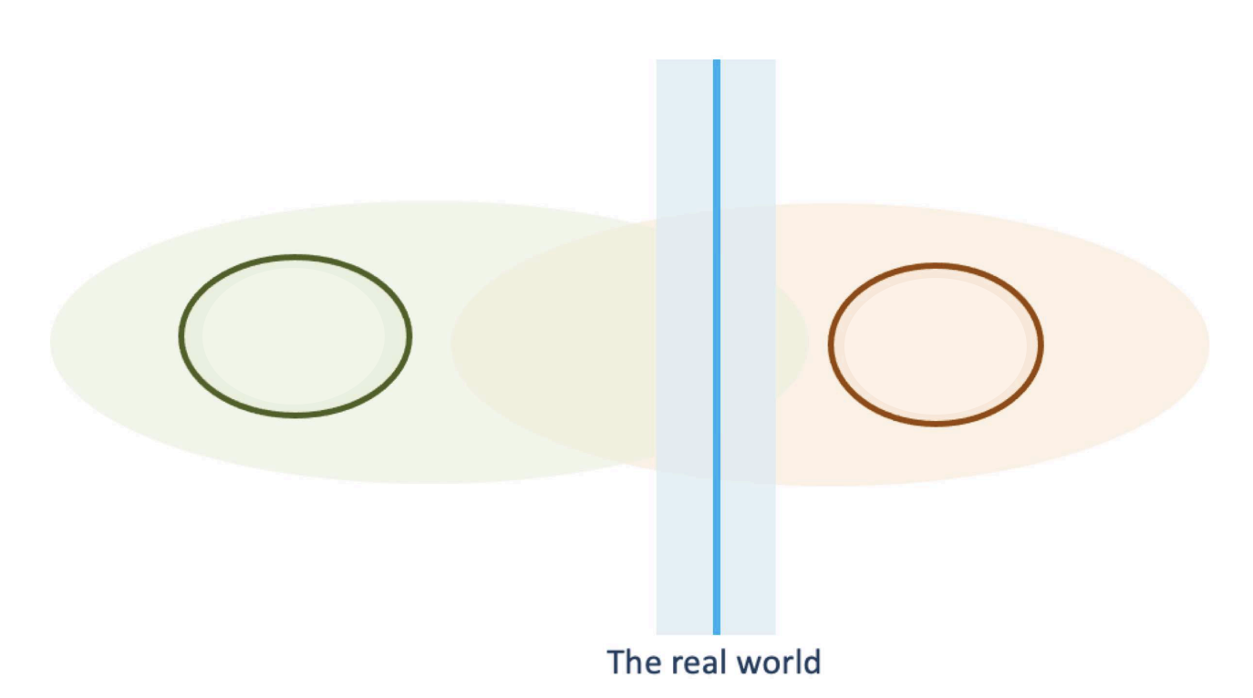
The green circle is

Mode: deterministic

The red circle is

Chaos: stochastic climate

El Nino originated in

South American fisheries

Southern Oscillation

Pressure difference between Tahiti and Darwin

ENSO coupling origin

Bjerknes identified the relation and suggested that this may account for variability in both

ENSO numerical model origin

Cane and Zebiak determined that an ocean and atmospheric model could reproduce the ENSO mode

The El Nino

Peaks around November to January, warming

ENSO events are marked by a

SST pattern in the tropical pacific

La Nina

Not as strong as warming events, last longer, intensification of the mean state

ENSO lasts for

2-7 years (4 average)

ENSO dynamics are controlled by

Dynamics in the upper ocean tropical Pacific

Thermocline

Strongest ENSO variability, region of the upper ocean where the temperature decreases very quickly (change from light/warm surface water to dense/cold subsurface waters)

Deepening of the thermocline marks

Increased heat content before an El Nino event in the western/central equatorial Pacific, propagates to the east, followed by large-scale surface warming

During strong surface warming, western thermocline marks

Reduced heat content, which propagates to the east, introducing the La Nina event

Prominent teleconnection of ENSO

Reduced Indian monsoon and reduced hurricanes during El Nino

Tropical pacific mean state is marked by

A strong temperature gradient from east (cold) to west (warm)

Equatorial cold tongue

Result of prevailing easterly trade winds (Hadley cell induced boundary conditions) and the Ekman ocean currents induced by friction and Coriolis forcing

Easterly winds lead to

Pile up of warm water and higher sea level on the western side

The thermocline has an

East to west gradient

Coriolis forcing results in _ at the equator

Divergence

Walker circulation

Secondary tropical circulation, with rising over the western warm pool and cooling over eastern equatorial Pacific.

Walker circulation results in _ surface pressure in the west and _ surface pressure in the east

Low, high

Bjerknes feedback: SST forces zonal wind

Warm SST causes heating in the atmosphere, low surface pressure and a reduced zonal easterly wind

Bjerknes feedback: Zonal wind forces thermocline

Easterly zonal winds keep the western Pacific thermocline deeper, weakening leads to a shallowing of the thermocline which propagates to the east.

Bjerknes feedback: Thermocline forces SST

A deeper thermocline in the east reduces the upwelling of cold subsurface waters along the equator and the south American coasts, leading to warming of SST.

Thermohaline circulation

Deep ocean circulation that spans the global oceans

Reduced North Atlantic MOC during warming is due to

Reduced temperature gradients between tropics and polar regions and poles warm more strongly

Density differences between two boxes in the Stommel model are controlled by

Temperature and salinity differences

If temperature differences dominate in the Stommel model

Surface flow is from the equatorial box to the polar box, reducing temperature gradients

If salinity differences dominate in the Stommel model

Surface flow is from the polar box to the equatorial box, reducing the temperature in the equatorial box

Proxy data

Data from the past climate not related to direct measurements.

Milankovitch cycles

Cause the glacial cycles dominating the last 500,000 years, with warm periods every 100,000 years

The biggest driver of ice age cycles is most likely

Variations in earth’s orbit around the sun, caused by other planets and the moon (milankovitch cycles)

Glacier feedbacks

Ice albedo, water vapour, altitude cooling and atmospheric circulation

Ocean CO₂ uptake feedback

Cold oceans can uptake more CO₂ than warm oceans.

Eccentricity

The shape of the earth’s orbit around the sun

Precession

The position of the seasons within the orbit around the sun

Obliquity

Changes in the angle of tilt of Earth’s axis rotation