ECON 102 Final

Economic Rent

* paying for the use of any resource above its opportunity cost


* Largest when:
* resources can’t be replicated
* little competition
* goods/services are allocated to resources that place the highest value on them

Accounting profit

* the actual amount of money a company earns during a given period. If 0, there is no profit

Economic profit

* Will always ≤ accounting profit.


* If 0, you are earning as much as you could at your next-best alternative

Economic Profits As Signals

* Negative: you could earn more money elsewhere, exit the industry
* Positive: your firm/industry is doing well, others should enter
* Zero: you are doing as well as you could elsewhere, but you could do just as well doing something else, don’t exit or enter

Total revenue (TR)

P x Q

Profit (π)

TR - TC

Short run vs long run

* Short run: capital is fixed input
* Long run: all factors of production can be varied, except for the current level of technology

Marginal principle

* If MR > MC, produce more
* If MR < MC, reduce to MR = MC
* If MR = MC, optimal level of production where profit is maximized

Total product (TP)

the total amount of output produced

Average product labor (APL) and Average product capital (APK)

* APL = TP/L
* APK = TP/K

Marginal product labor (MPL)/marginal product capital (MPK)

* the change in total output that results from using one more unit of an input
* MPL = ΔTP/ΔL
* MPK = ΔTP/ΔK

Diminishing MPL vs diminishing APL

Initially the MPL/APL will increase with each additional unit of labor we add; however, when adding a worker has a positive MPL but lower than the previous worker’s MPL - diminishing marginal productivity/when the average number of units we produce per laborer starts to decrease - diminishing average productivity

If MPL > APL, APL curve?

If MPL < APL, APL curve?

* APL curve will slope upward
* diminishing APL starts and slope downward

Total fixed costs (TFC)

constant at all activity levels within the relevant range, horizontal graph

Total variable costs (TVC)

changes in direct proportion to the number of units produced in the relevant range, always at the origin, positive linear graph

Total costs

changes in direct proportion to the number of units produced due to variable costs, positive linear graph above the origin, y-intercept = FC

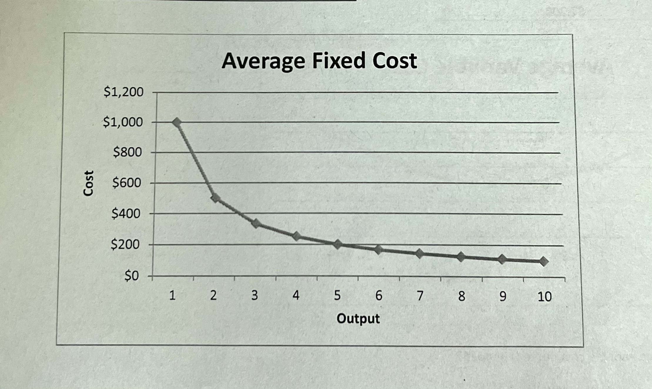
Average Fixed Costs (AFC)

fixed costs allocated to each unit produced, always decreasing as we produce more units b/c allocating TFC among more units while it’s constant

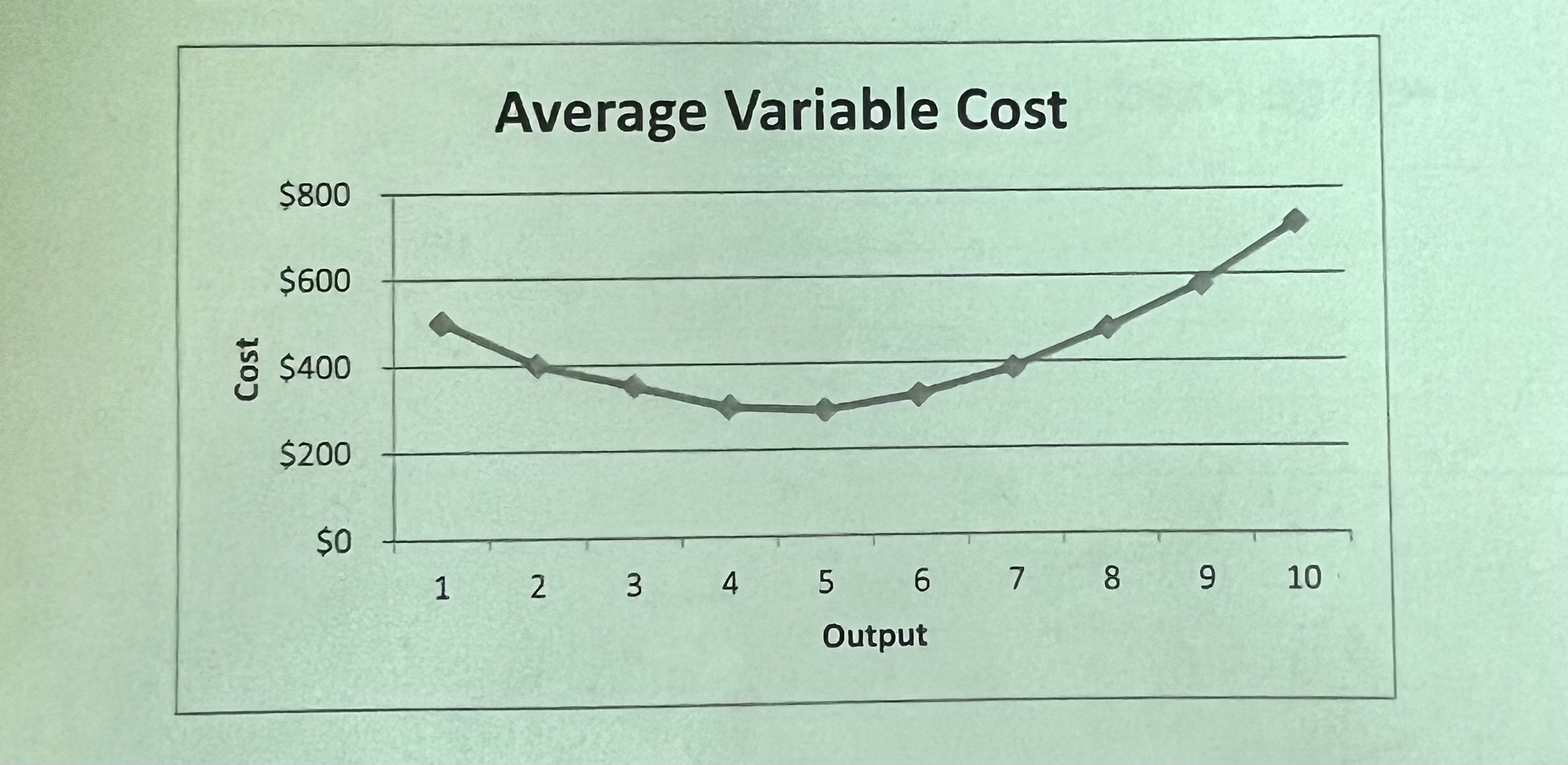
Average Variable Costs (AVC)

* variable costs allocated to each unit produced


* U-shaped b/c initially more efficient when we produce more units, but as resources get stretched producing more units becomes inefficient causing the additional variable cost per unit to increase

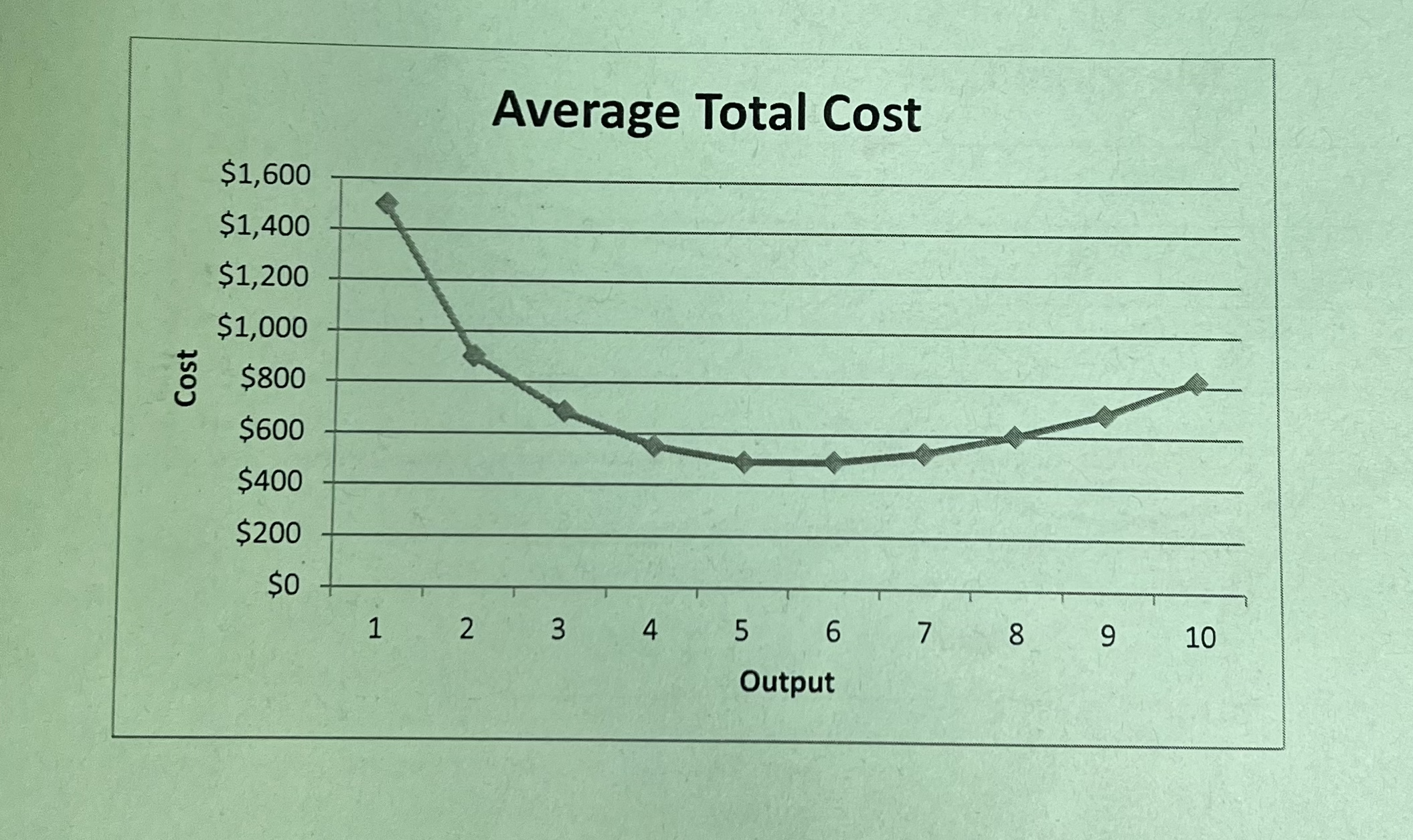
Average Total Cost (ATC)

* total cost allocated to each unit produced - on average, how much it costs or produce a unit of output


* U-shaped b/c AVC is part of ATC

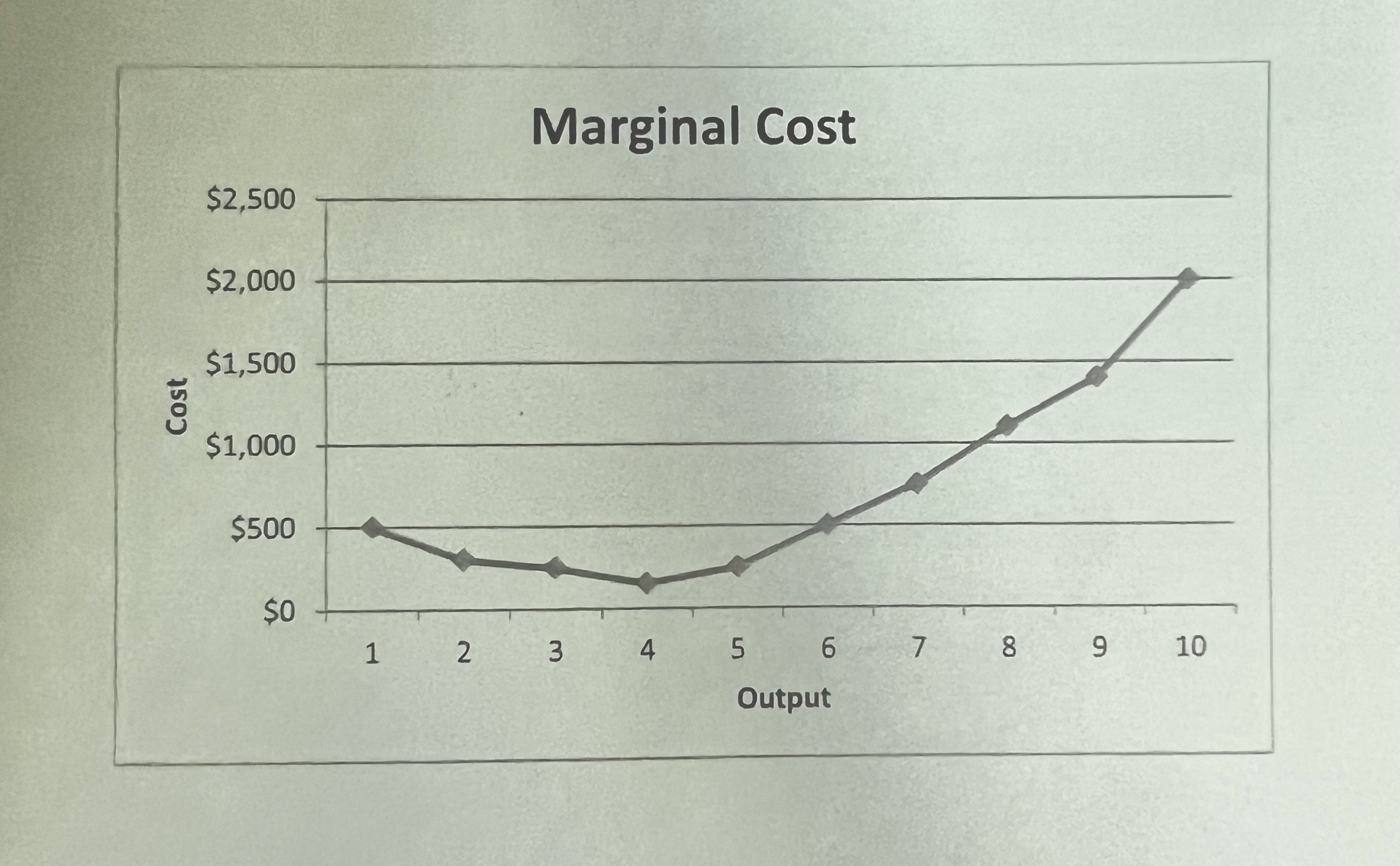
Marginal cost

U-shaped b/c the cost of producing an additional unit will increase as more are produced

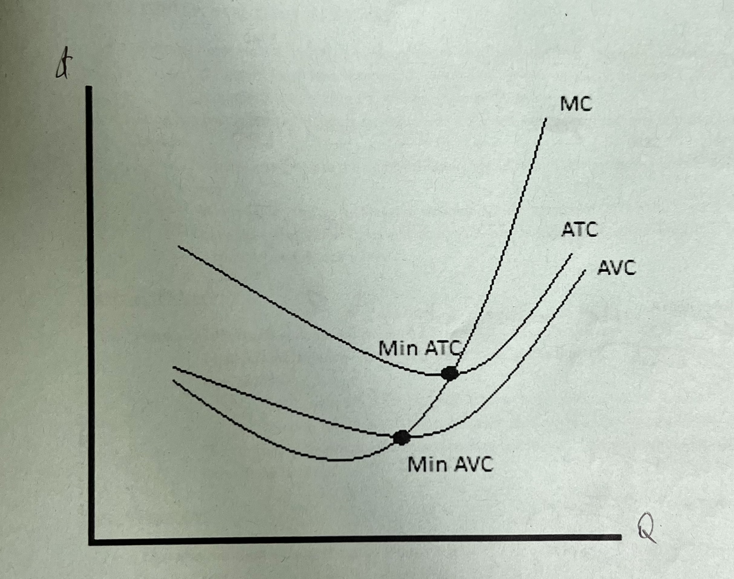
Relationship between ATC, AVC, and MC

* MC always intersects the min point of ATC and AVC
* If MC < ATC, ATC decreases
* If MC < AVC, AVC decreases
* If MC > ATC, ATC increases
* If MC > AVC, AVC increases

Cost minimization

* using the production method that produces a given level of output at the lowest possible cost, profit max = cost min
* Assume horizontal L and K supply curves, so prices of additional units of L and K are constant
* Assume MP changes as we use more or less L or K

Long run cost curve

* the lowest cost of producing each level of output when all inputs can be varied
* No difference b/w ATC, AVC, and AFC b/c no fixed costs so all are variable
* MC increases faster in short than long b/c fixed capital in short run
* Short run never fall below LRAC b/c it shows lowest cost for each output level
* Optimal level of inputs b/c no fixed inputs, unlike short run

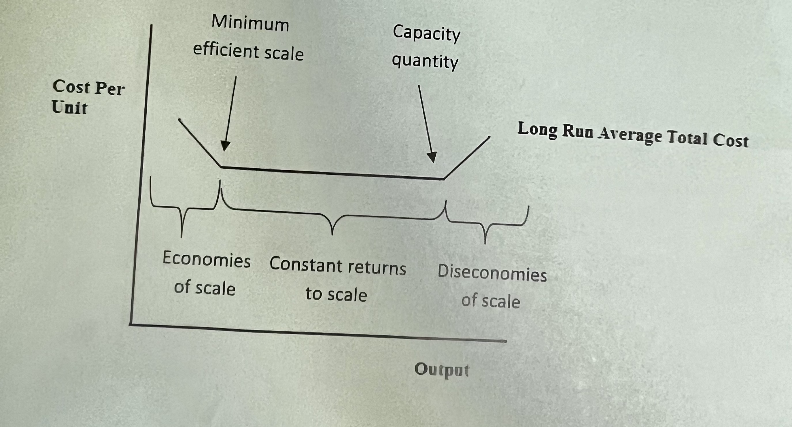
Minimum efficient scale (MES)

the first point of production where ATC is lowest for a firm

Small vs Large MES

* Small: only a small amount of output needed, resulting in many efficient firms and lots of competition
* Large: large amount of output needed, resulting in a small number of efficient firms and little competition

Capacity quantity

the last point of production where ATC is the lowest for a particular firm

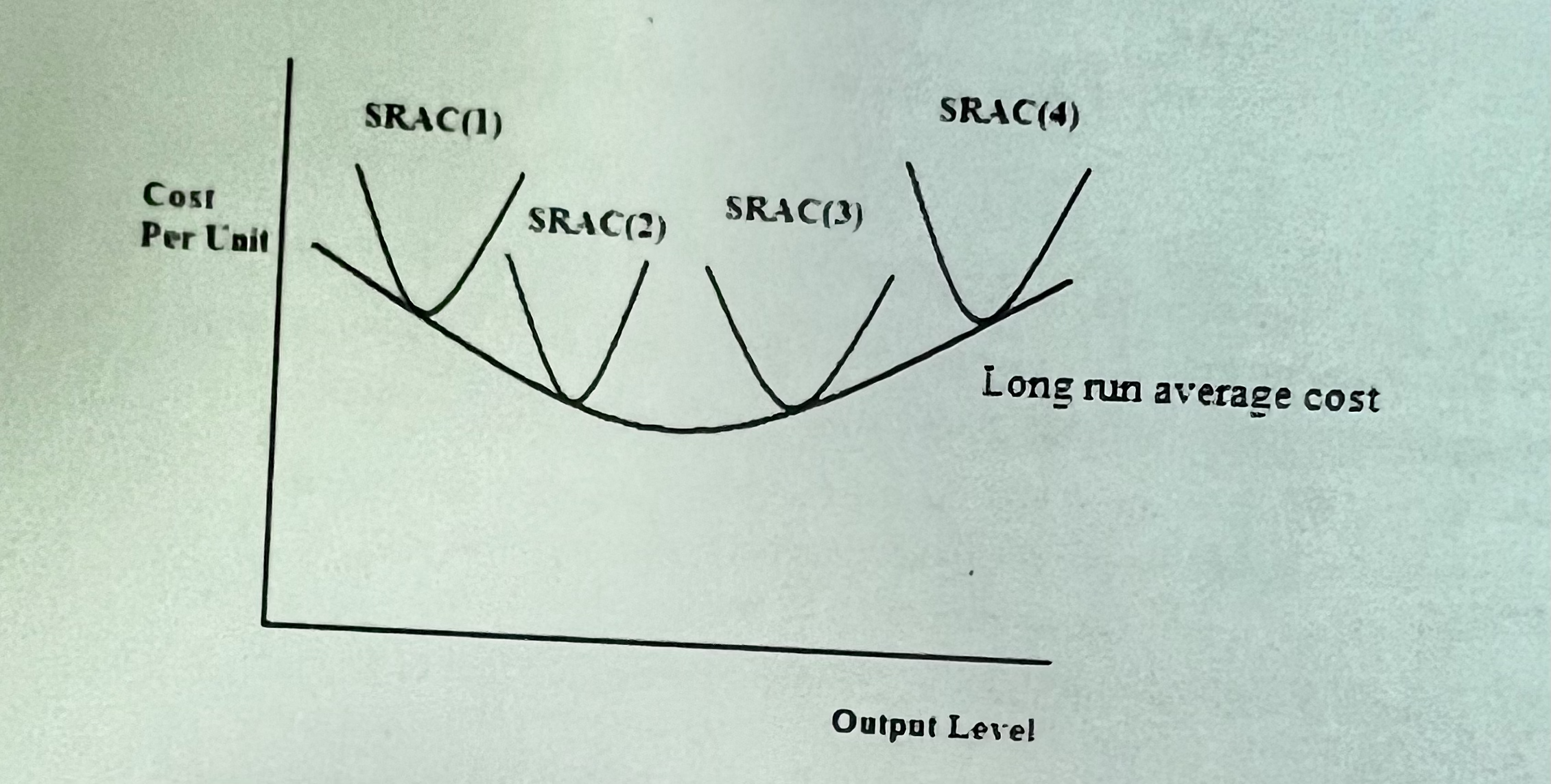
Long run average cost curve (LRAC)

shows the lowest possible cost for each output level

Economies of scale

* ATC decrease as we produce more units
* doubling the inputs more than doubles the output
* In the range of production, increasing output allows for more efficient use of inputs
* occurs at smaller levels of output and will eventually slow down as output increases

Constant returns to scale

* no change in ATC as we produce more units
* doubling inputs exactly doubles output
* plant is at the ideal size

Diseconomies of scale

* ATC increases as we produce more
* doubling inputs less than doubles output


* In this range of production, high levels of output results in less efficient use of inputs

Reasons for economies of scale

* specialization
* improvement in production equipment

Reasons for diseconomies of scale

* more output = larger plant size = larger firm size
* adding layers of management
* decrease in flexibility

Relationship b/w SRATC and LRAC

* point of SRATC that’s tangent to LRAC is where the output in the short run reaches min LRAC for the amount of the fixed input in the short run
* SRATC is steeper than LRAC when increasing output b/c firms need to make inefficient choices in the short run since one of their inputs is fixed

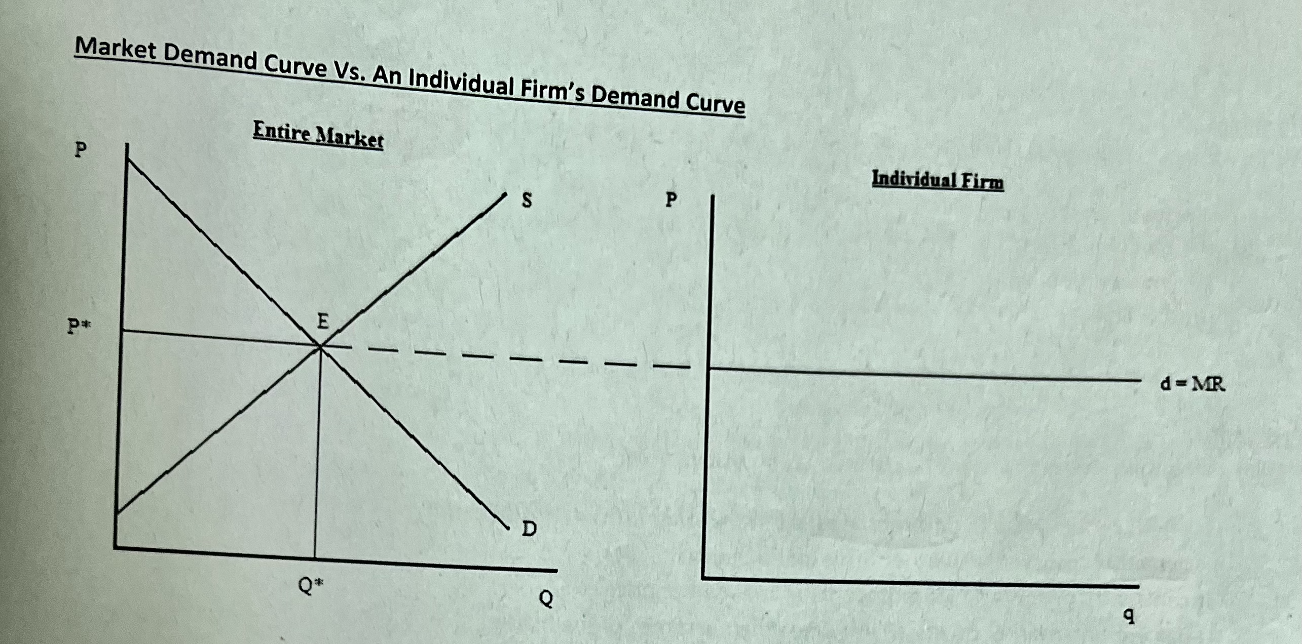
Entire market/industry graph and individual firm graph

demand curve is downward sloping for the industry/perfectly elastic demand curve

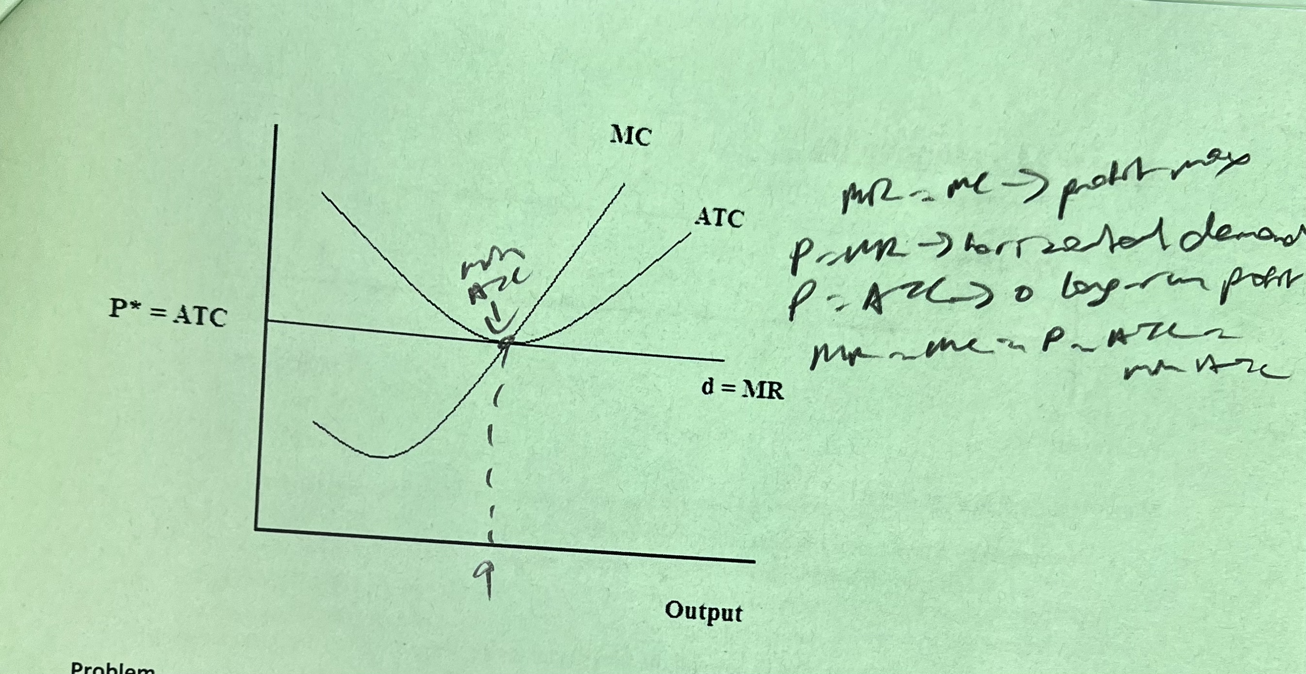
Profit maximizing rule

firms max profit at MR = MC for all market structures

Marginal revenue (MR)

* the incremental change in revenue when we sell one more unit
* MR = ΔTR/Δq

Short run: continue to operate vs shut down

* If P > min(ATC), continue to operate b/c positive economic profit
* If P = min(ATC), continue to operate b/c zero economic profit (long run equilibrium for perfect competition)
* If min(AVC) ≤ P < ATC, continue to operate in the short run with a loss
* If P < min (AVC), shut down

Short run economic profit

* If positive profit, more firms enter, causing the supply curve to shift to the right, causing prices to fall until economic profits are zero
* If negative profit, firms exit, causing the supply curve to shift to the left, causing prices to rise until economic profits are zero

Conditions for long run equilibrium in perfect competition

* each firm max profits at P = MR = MC
* Economic profit = zero
* no entry/exit

Types of Barriers to Entry in Monopolies

* ownership of resources w/o substitutes
* economies of scale: when the cost of production goes down a lot as more is produced it’s harder for small companies to compete w/ monopolies b/c the monopolies per unit cost is so much lower
* government licensing

Ways Government Legislation Creates Monopolies

* licenses and franchises
* patents
* tariffs
* regulations
* quality standards

Ways firms create barriers to entry

* buying up all available resources
* increasing competitor’s costs
* threats of sabotage
* predatory pricing

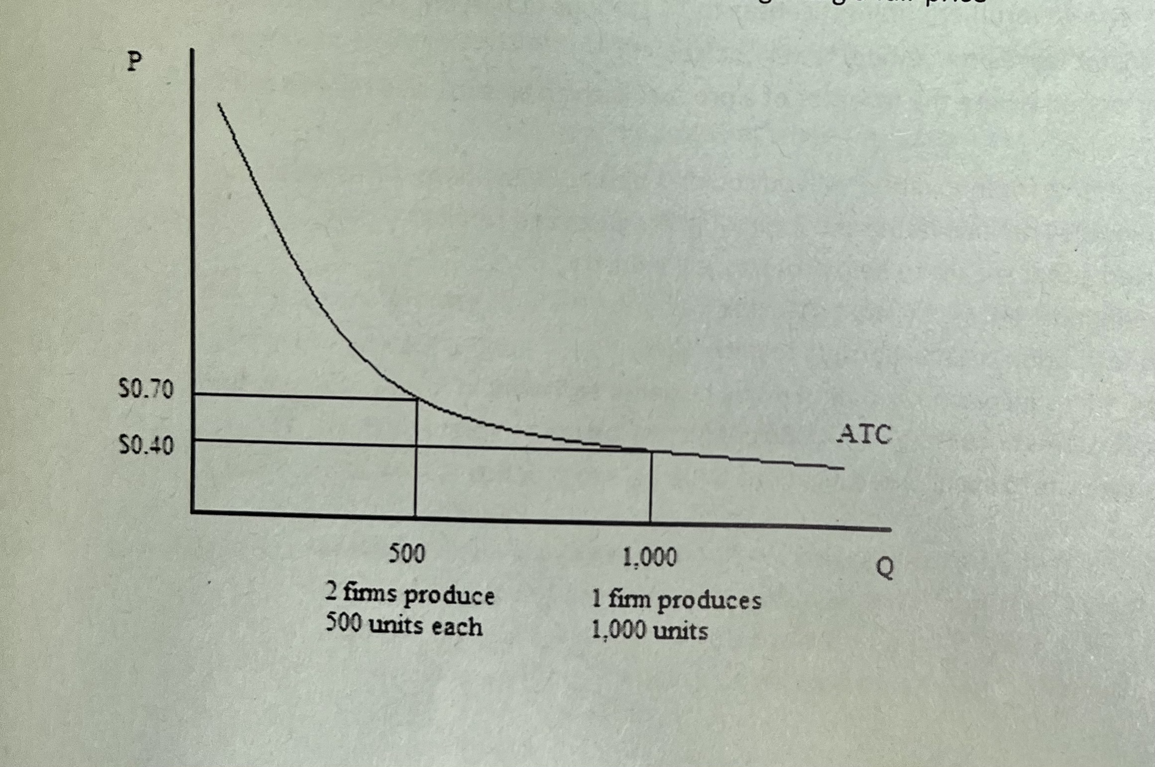
Natural monopolies

* a firm has decreasing ATC over a large range of output, ex: electric companies
* occur in industries w/ high FC
* Large firms are more efficient than small ones due to EoS b/c larger firm can drive out others by cutting their prices

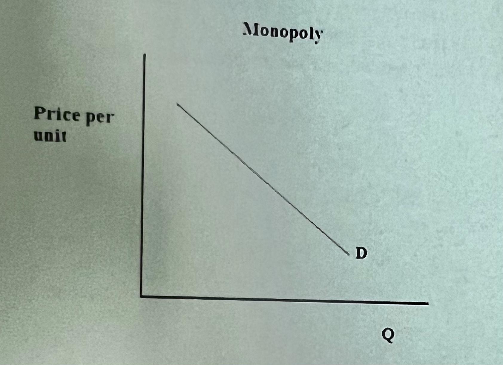
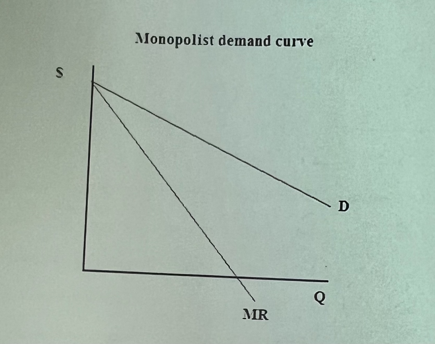
Monopolist’s demand curve

* same as market demand curve b/c one firm is the entire market
* also = monopolist average revenue (AR) curve b/c price is determined by the position of the demand curve

MR for monopolists

Produce where P > (MR = MC) b/c a monopolist’s MR curve is twice as steep as its demand curve

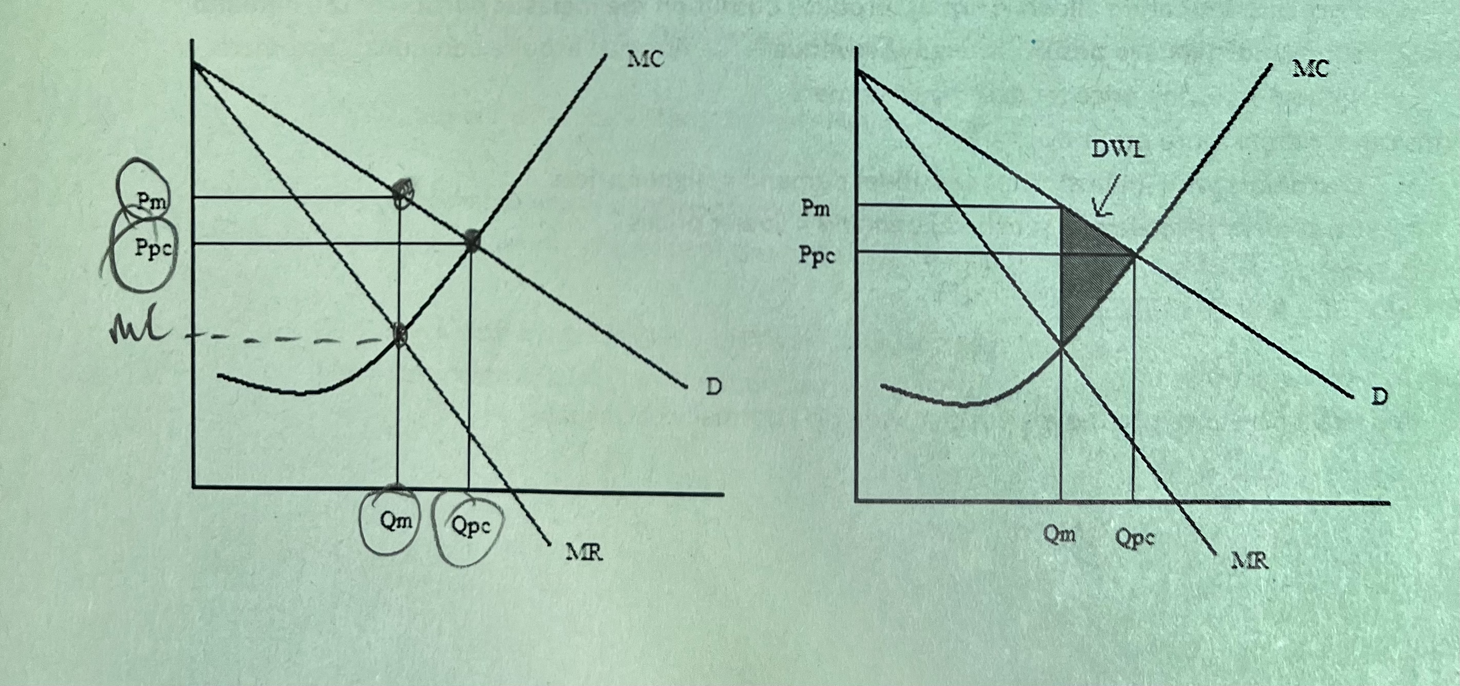
DWL for monopolies

* B/c monopolists produce where P > (MR = MC)
* Monopoly price > perfect competition price - consumers pay higher prices
* monopoly quantity < perfect competition quantity - fewer units available for consumers

Price discrimination

when a business sells the same product at different prices for reasons unrelated to cost, allowing them to produce output on the inelastic portion of the demand curve but still have positive MR

Conditions to Price Discriminate

* firm has a downward sloping demand curve
* firm must easily and cheaply identify customers with predictably different elasticities of demand
* arbitrage opportunities can’t exist

Arbitrage

when consumers buy a good at a low price and then resell it to other consumers at a high price

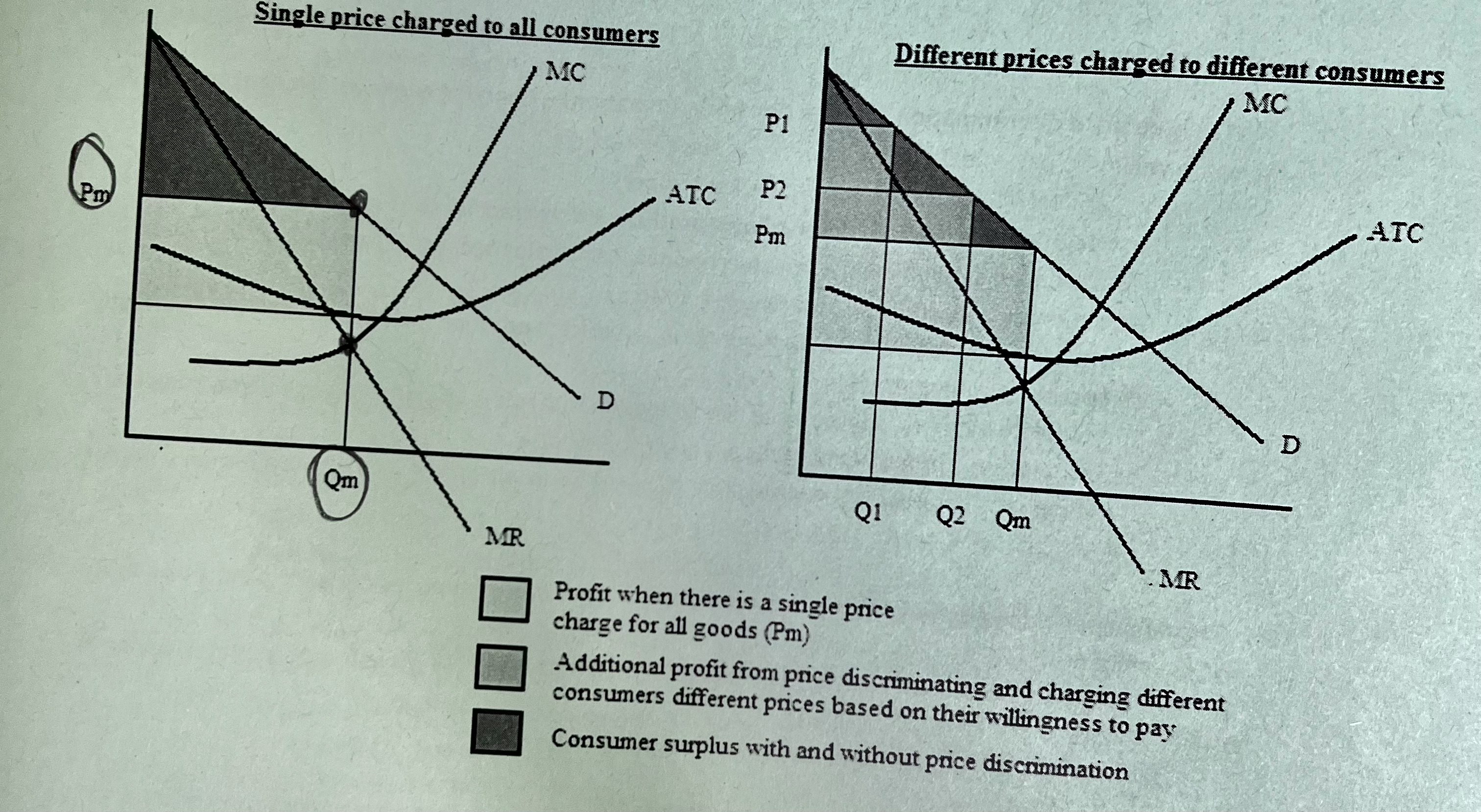
First degree price discrimination (perfect price discrimination)

* charging every customer exactly what they’re willing to pay, allowing producers to extract all consumer surplus, meaning it’s efficient b/c no DWL since last unit is sold at P = MC
* producers produce the best possible (perfectly competitive) output level
* inequitable b/c some are paying a lot while others pay little

Second degree price discrimination

* customers are charged different prices depending on the quantity they purchase
* larger quantities = better price

Third degree price discrimination (market segmentation)

* when a firm can segment consumers in different groups based on the elasticity of their demand and charge them different prices
* customers w/ inelastic (not sensitive) demand, higher prices
* customers w/ elastic (sensitive) demand, lower prices

Effect of market segmentation on the monopoly graph

effective price discrimination = higher profits than single price

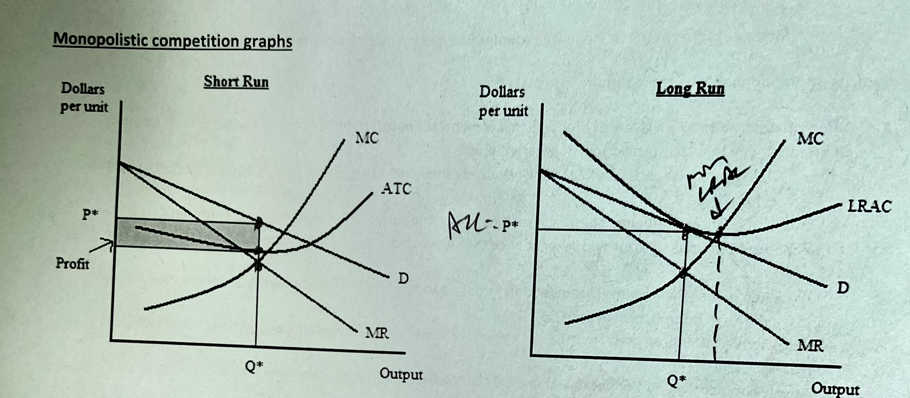
Profit maximization in monopolistic competition

* profit max at MR = MC
* short run: firms can earn profit/losses
* long run: zero profit and excess capacity

Excess capacity in monopolistic competition

* In the long-run equilibrium, goods are produced at a point where ATC is not at a min
* doesn’t mean waste if consumers are willing to pay higher prices for product variety

Prices vs Quantity for competition, monopolistic competition, and monopoly

* Price: perfect competition < monopolistic competition < monopoly
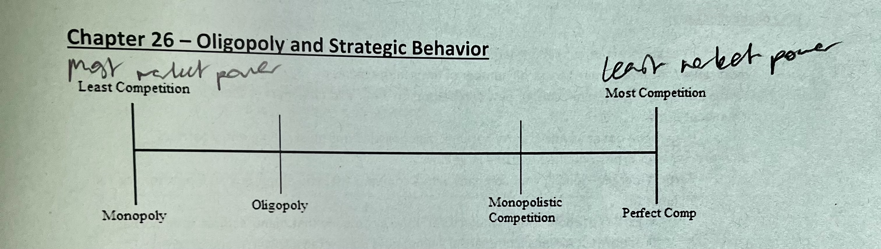
* Quantity: monopoly < monopolistic competition < perfect competition
* Perfect competition is best for consumers and monopoly is the worst for consumers

Oligopoly

* an industry containing two or more firms and at least one produces a significant portion of the industry’s total output
* firms consider the actions of their competitors when setting price

Reasons Oligopolies Occur

* Economies of scale: in some markets larger firms are more efficient than small firms, so there would be only a small number of firms in the market
* barriers to entry: if there aren’t any natural ones, oligopolistic firms need to create them
* mergers
* vertical merger: joining your company with another that you either buy an input from or sell an input to
* Horizontal merger: joining your company with another that sells a similar product

Types of Entry Barriers in Oligopolies

* Brand proliferation: if a large number of differentiated products already exist, little room for new firms to take


* advertising: if a firm already in the market advertises heavily, a firm wanting to enter also would have to advertise heavily, increasing their cost
* if that firm has a low MES, the additional advertising costs could result in a higher MES for them which could prevent them from entering

Industry concentration ratios

* measure economic power in an industry and shows the market share of the industry’s largest firms
* If high (close to 100%), it’s very concentrated with little competition
* If low (close to 0%), no firm has a significant share and lots of competition

Four firm concentration ratio

TR for 4 largest firms/TR for all firms

Herfindahl-Hirschman Index (HHI)

a better way to measure industry concentraion that takes into accont when a single firm dominates an industry

Σ i=1 to N, si^2

Sales share percentage (si)

Firm’s revenue/TR for all firms

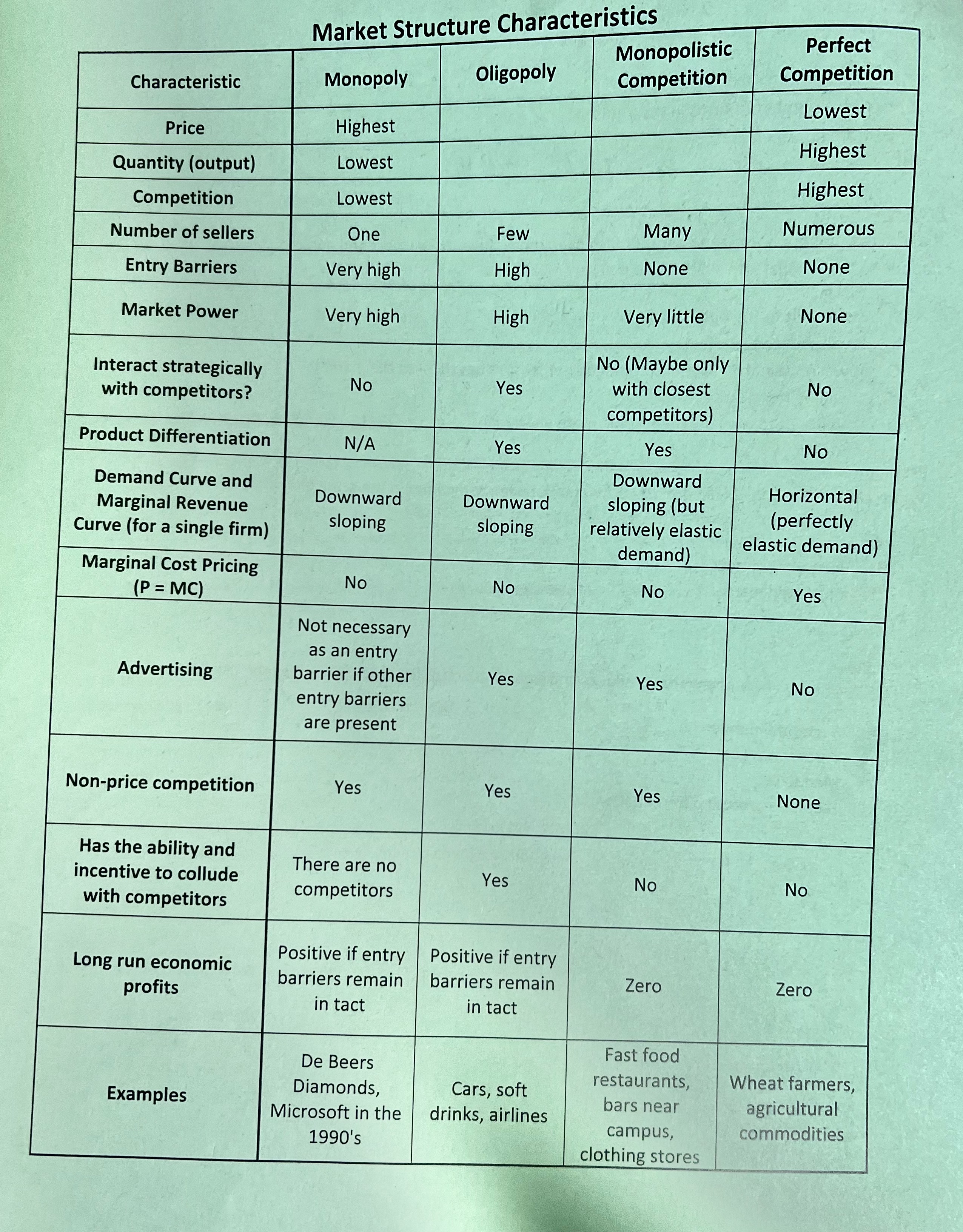
Market structure characteristics