A Level Biology Paper 3: General Exam Flashcards

• Mix each dilution.

• Repeat plating and calculate a mean.

• Take photo of final plate so colonies can be counted.

• Reduce number of dilutions.

Name a common error in serial dilution that leads to an overestimate.

• Failure to change pipette tips between steps, causing "carry-over" of extra bacteria into subsequent tubes.

Data collected

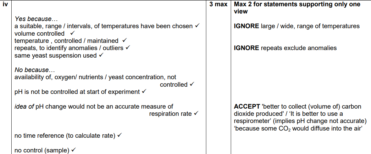
• Appropriate range of temperatures, which are controlled in a thermostatically controlled room.

• At least three repeats, identification of anomalies and calculate means, as well as standard deviation.

Valid control

• Area of leaf

• Humidity

• Light Intensity

• Same plant

• Air movement

• Time

Statistical Test

• Spearman’s rank.

List 4 controlled variables for a transpiration temperature experiment.

1. Light Intensity (kept constant with a lamp at a fixed distance).

2. Humidity (monitored with a hygrometer).

3. Air Movement/Wind (no fans/drafts).

4. Total Leaf Area (use the same plant cutting throughout).

When is Spearman’s Rank used vs. a t-test in biology?

Use Spearman’s Rank to look for a correlation between two continuous variables (e.g., temperature and rate). Use a t-test to look for a significant difference between two means (e.g., rate at 20°C vs. rate at 30°C).

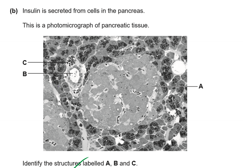
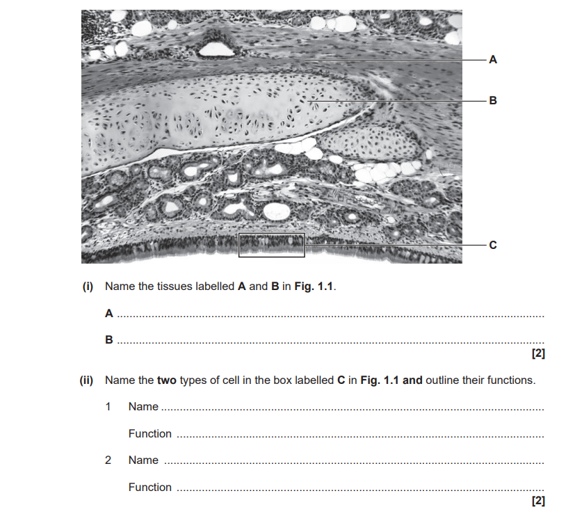
• A: Islets of Lagerhans

• B: Duct

• C: Blood vessel

• Marker

• Gene for antibiotic resistance

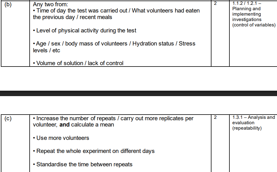
Repeatability refers to getting the same results when the same student repeats the experiment under the same conditions. To score the 2 marks, you must suggest ways to tightly standardise the method:

• Standardise the physical activity during the 2-hour testing window (e.g., require all volunteers to sit still or remain at rest throughout the test).

• Ensure the same overnight fasting time is strictly kept for all repeats and individuals.

• Dissolve the glucose in a fixed, controlled volume of water each time.

• Ensure the volunteers consume the drink in a set timeframe (e.g., within 5 minutes).

• Use volunteers of identical profiles (e.g., same age, sex, and BMI category) for any subsequent experimental groups.

Key Terminology Distinction: Be careful not to confuse repeatability with reproducibility or simply increasing sample size. While testing a larger number of volunteers improves the overall reliability of the data, the specific command word repeatability requires you to refine the protocol so that a single worker can achieve consistent results every time they replicate the trial.

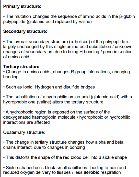
To answer this question perfectly, you must systematically address the primary, secondary, tertiary, and quaternary structures before explaining how these changes generate the physiological symptoms.

Mark Scheme Answers1. Primary Structure

• The sequence / order of amino acids is altered. * Specifically, the hydrophilic amino acid glutamic acid is replaced by the hydrophobic amino acid valine at position 6 in the $\beta$-globin polypeptide chain.

2. Secondary Structure

• The folding of the local polypeptide chain is altered.

• The distribution of hydrogen bonds changes, which can slightly disrupt or misfold the normal configuration of alpha-helices and beta-pleated sheets.

3. Tertiary Structure

• The overall 3D shape / conformation of the single beta-globin subunit is altered.

• This is because the substitution introduces valine, which has a hydrophobic R-group.

• This changes the hydrophobic and hydrophilic interactions (and potentially ionic/hydrogen bonds) within the protein, causing a hydrophobic patch to form on the outside of the molecule.

4. Quaternary Structure

• The interaction between multiple polypeptide subunits is altered.

• Haemoglobin is a conjugated globular protein made of four subunits (alpha and beta).

• In deoxygenated sickle haemoglobin (HbS), the external hydrophobic valine patch binds to a complementary hydrophobic patch on a neighbouring haemoglobin molecule.

• This causes the individual haemoglobin molecules to aggregate, polymerise, or stick together to form long, insoluble fibres/strands.

5. Link to Symptoms

• The long molecular fibres distort the normal biconcave shape of the red blood cell into a rigid, sickle shape.

• These rigid cells cannot easily flex through narrow capillaries, leading to blockages in small blood vessels.

• This cuts off blood supply to tissues, causing localized oxygen deprivation, tissue damage, severe pain (sickle crisis), and reduced overall oxygen delivery (anaemia).

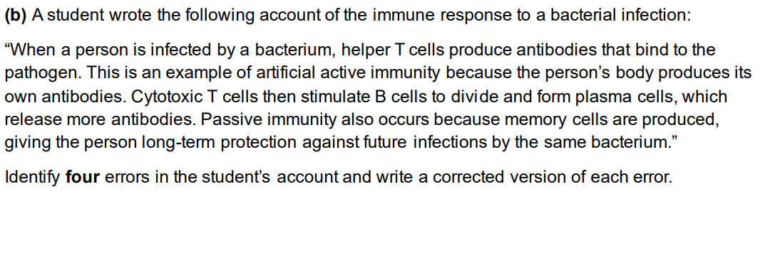
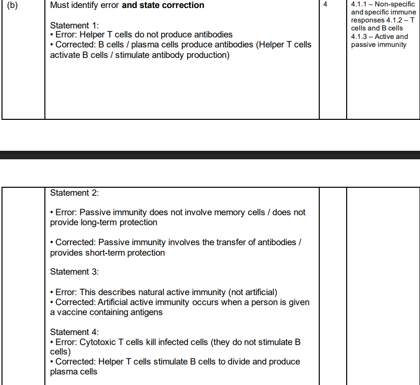
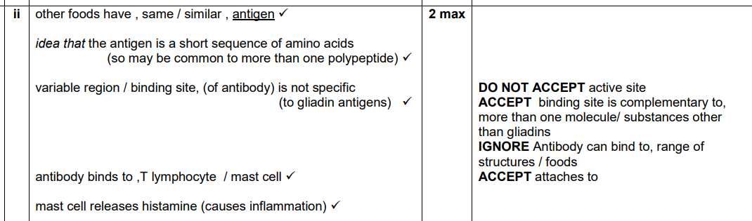
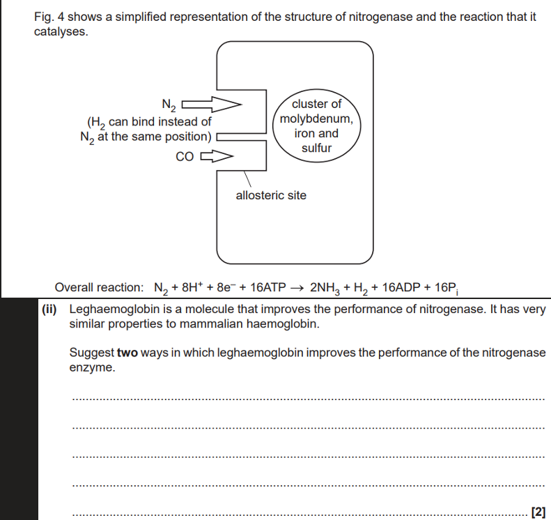
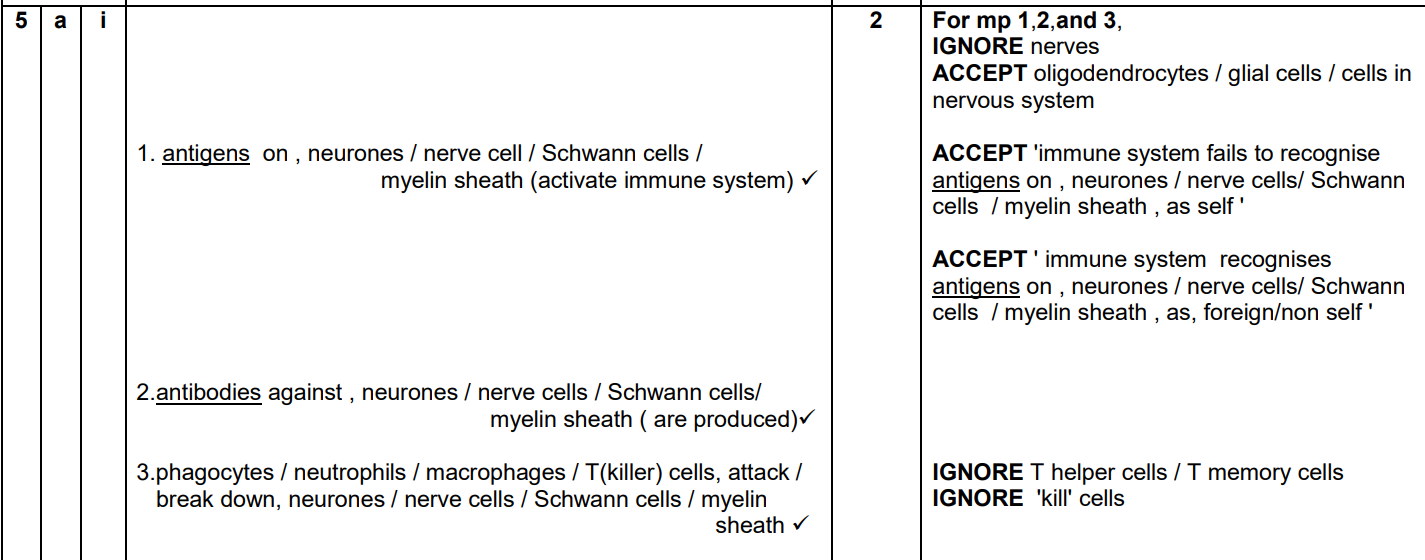
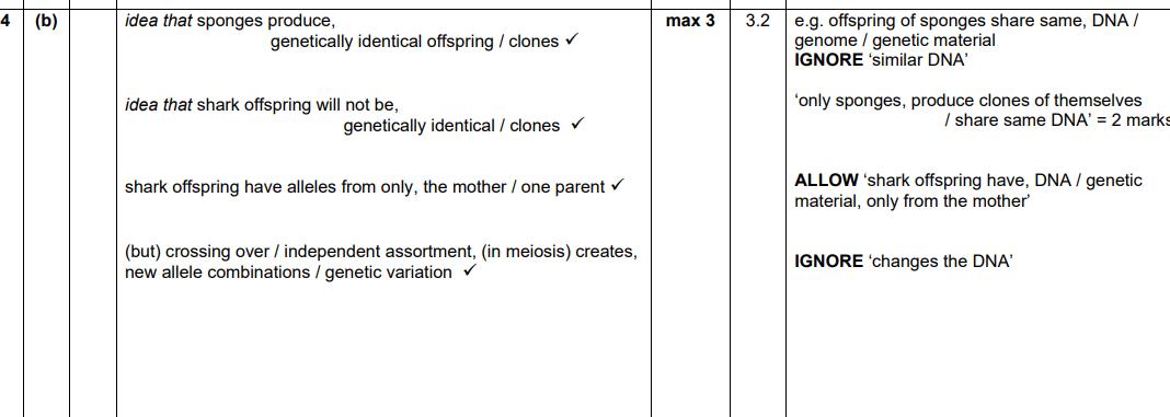
The Four Identified Errors and Their CorrectionsError 1: The cell that produces antibodies

• The Student's Claim: "...helper T cells produce antibodies..."

• The Correction: Helper T cells do not produce antibodies. Antibodies are produced and released exclusively by plasma cells (which differentiate from activated B lymphocytes). Helper T cells instead release interleukins/cytokines to activate these B cells.

Error 2: The classification of immunity from an infection

• The Student's Claim: This is an example of "artificial active immunity"

• The Correction: Catching a disease from a live pathogen is a natural environmental exposure, making it an example of natural active immunity. "Artificial active immunity" is only achieved via medical intervention, such as receiving a vaccination.

Error 3: The cell that stimulates B cell division

• The Student's Claim: "Cytotoxic T cells then stimulate B cells to divide..."

• The Correction: Helper T cells are the cells responsible for stimulating B cells to undergo clonal expansion and differentiation. Cytotoxic T cells (or T-killer cells) function to directly destroy infected host cells.

Error 4: The role of memory cells in classification of immunity

• The Student's Claim: "Passive immunity also occurs because memory cells are produced..."

• The Correction: The production of memory cells (B and T memory cells) is a hallmark feature of active immunity. Passive immunity involves a person receiving pre-made antibodies from an external source (e.g., across the placenta or via an injection), meaning no memory cells are produced and the protection is strictly short-term.

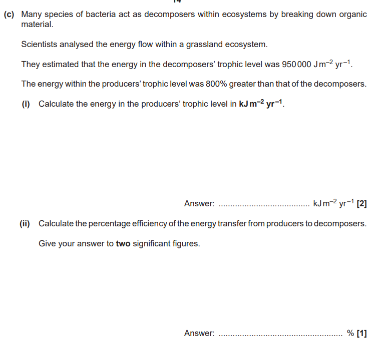
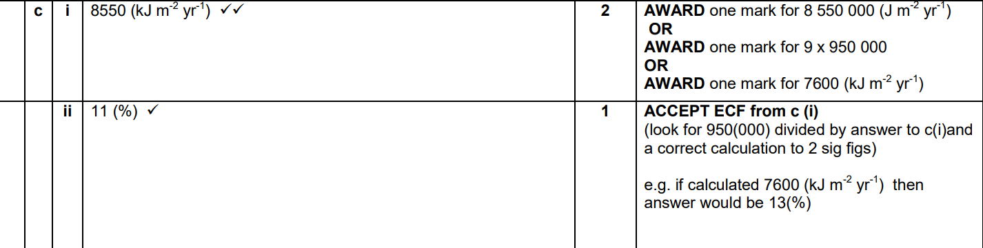
$\text{Energy in J} = 950,000 \times 9 = 8,550,000\text{ J m}^{-2}\text{ yr}^{-1}$1

$$\text{Energy in kJ} = \frac{8,550,000}{1000} = \mathbf{8550}$$

$$\text{Efficiency} = \frac{\text{Energy in receiving trophic level}}{\text{Energy in preceding trophic level}} \times 100$$

$$\text{Efficiency} = \frac{950,000}{8,550,000} \times 100 = 11.1111...\%$$

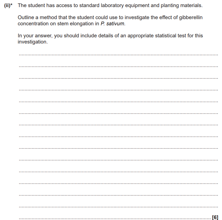
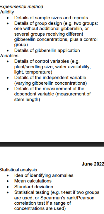
• dependent Variable ($IV$): Set up a range of at least 5 different gibberellin concentrations (e.g., $0\text{ ppm}, 10\text{ ppm}, 20\text{ ppm}, 30\text{ ppm}, 40\text{ ppm}$, and $50\text{ ppm}$). This range should be prepared via serial dilution of a stock gibberellin solution.

• Control Group: The $0\text{ ppm}$ group acts as your control. Treat these plants with plain distilled water containing no additional gibberellin to provide a baseline for natural stem elongation.

• Sample Size & Repeats: Use a large sample size of at least 10 to 20 P. sativum (pea) seedlings per concentration group. This ensures anomalies can be easily spotted and reduces the impact of genetic variation. Repeat the entire investigation on different days to ensure repeatability.

• Application Method: Apply a fixed, measured volume (e.g., $0.5\text{ cm}^3$) of each gibberellin concentration directly onto the apical bud or stem of each seedling using a micropipette at regular intervals over a set period (e.g., 2 weeks).

Section 2: Dependent Variable & Controlled Variables

• Dependent Variable ($DV$): Measure the stem length of each P. sativum seedling before the application begins and at regular intervals (e.g., every 2 days) using a millimeter ruler. Calculate the total change in stem elongation ($\text{final length} - \text{initial length}$) or the rate of elongation per day.

• Controlled Variables: To guarantee experimental validity, keep all environmental and physical factors strictly constant across all groups:

  • Initial seedling size/age: Ensure all pea seedlings are from the same batch, germinated at the same time, and are of a similar starting height.

  • Temperature: Keep all plants in the same room or growth incubator maintained at a constant temperature (e.g., $20^\circ\text{C}$).

  • Light availability: Expose all groups to identical photoperiods (e.g., 16 hours of light, 8 hours of dark) and light intensities.

  • Water and nutrient availability: Water each seedling with an equal volume of water daily and grow them in identical soil types within matching pots.

Section 3: Data Processing & Statistical Analysis

• Anomalies and Means: Inspect the raw data collected to identify and exclude any anomalies, then calculate the mean change in stem elongation for each of the gibberellin concentration groups.

• Standard Deviation: Calculate the standard deviation for each group to measure the spread of the data around the calculated means and to gauge data precision.

• Statistical Testing: * Because a continuous range of different gibberellin concentrations is being investigated, select and apply a Spearman’s rank correlation coefficient or a Pearson's linear correlation test.

  • This test will evaluate whether there is a statistically significant correlation between increasing gibberellin concentration and the degree of stem elongation in P. sativum, allowing you to confidently accept or reject your null hypothesis based on a critical values table ($p \le 0.05$).

  • (Note: If your design compared only two groups—one with gibberellin and a control group without—you would state that a Student's t-test should be used instead to compare the two means).

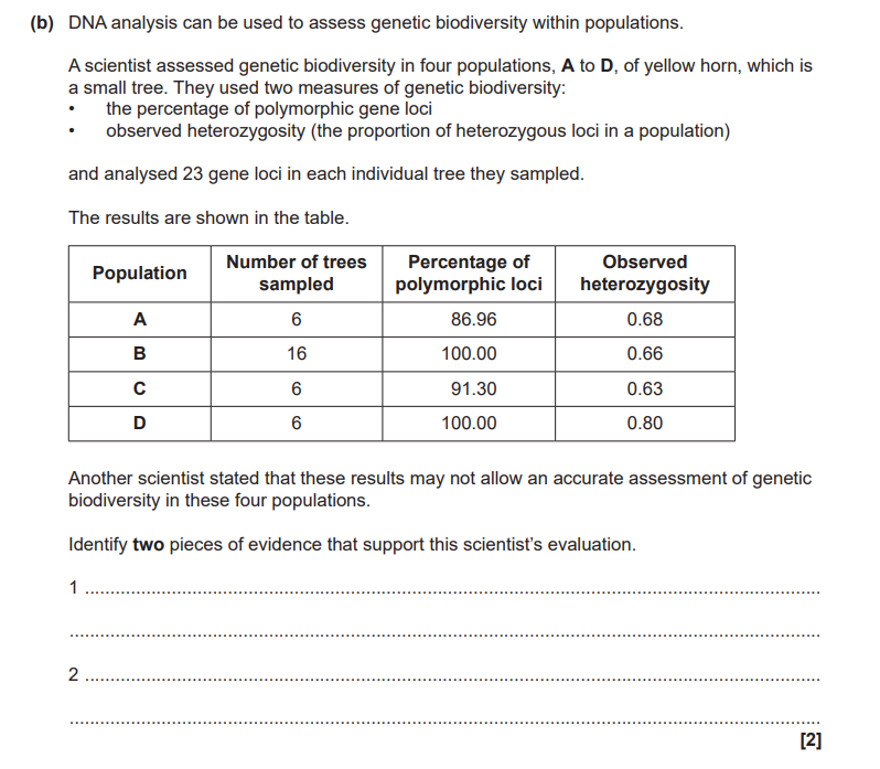
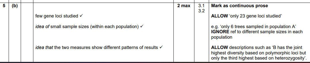
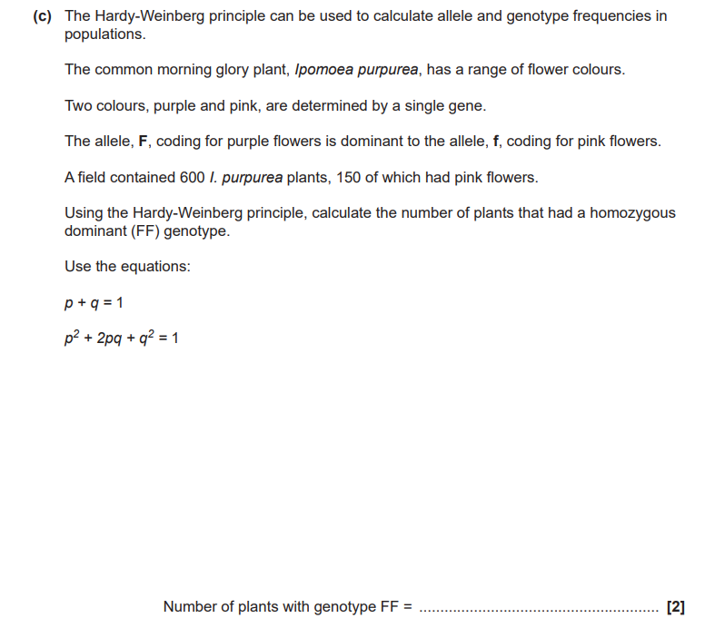
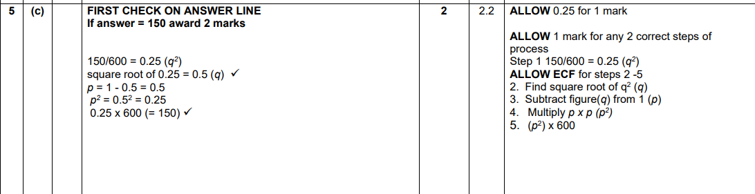
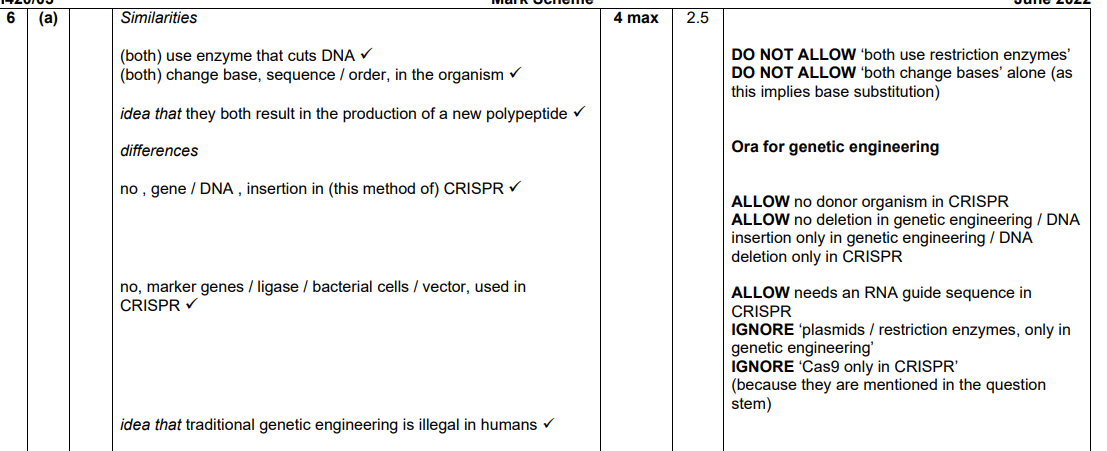
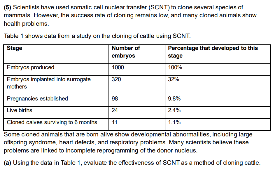
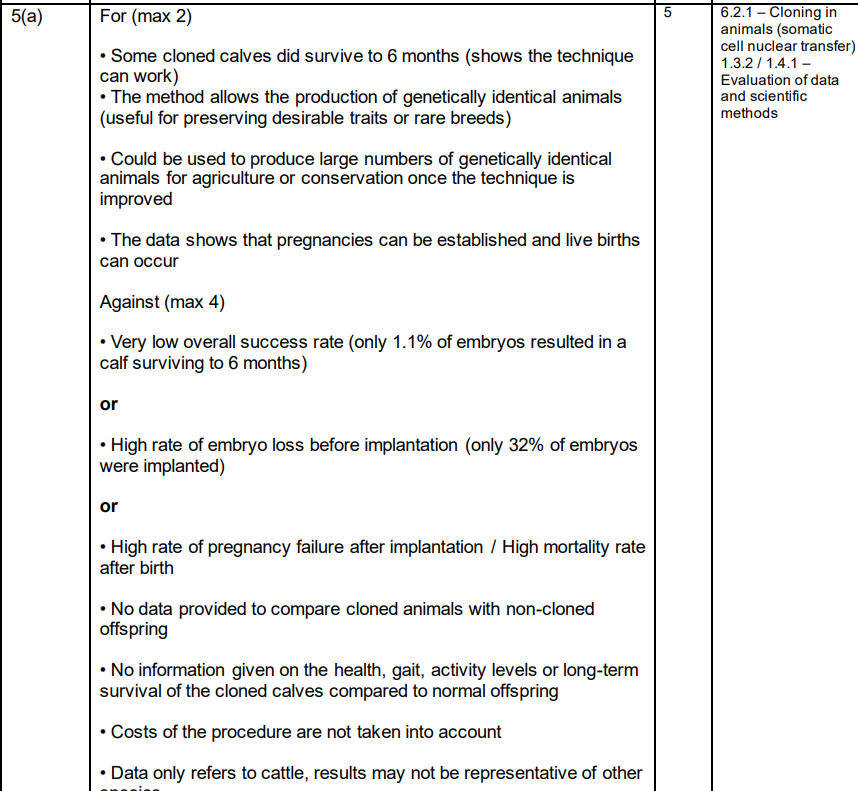
1. Small Sample Sizes (Number of trees sampled)

• Evidence: In populations A, C, and D, only 6 trees were sampled.

• Why this supports the evaluation: A sample size of 6 individuals is far too small to be representative of an entire tree population. It is highly susceptible to sampling bias and genetic drift, meaning any calculated biodiversity values are unlikely to reflect the true genetic diversity of the wider population.

2. Unequal / Inconsistent Sample Sizes

• Evidence: The number of trees sampled is not standardized across populations (population B has 16 trees sampled, whereas A, C, and D only have 6).

• Why this supports the evaluation: You cannot reliably compare genetic indices between populations when one group has nearly three times as many individuals sampled as the others. A larger sample size (like in population B) is inherently more likely to capture rare polymorphic loci, skewing comparisons.

3. Small Number of Gene Loci Investigated

• Evidence: The scientist analyzed only 23 gene loci in each individual tree.

• Why this supports the evaluation: A tree genome contains tens of thousands of active genes. Extrapolating the total genetic health and biodiversity of a species based on a tiny snapshot of just 23 loci is statistically weak and can easily produce an inaccurate overview.

When OCR asks you to evaluate why a study is inaccurate or unreliable, immediately check the first couple of columns in the data table. Examiners love to test your awareness of basic sampling rules:

• Always look for small sample sizes (typically anything under 10–20 repeats/samples is a major red flag).

• Check for unequal testing groups (unstandardized sample numbers break experimental validity).