Stats 5 Midterm

hi ryan

Census

we collect data for every individual in a population

Parameter

numerical summary of the population- values are usually unknown

Statistic

numerical summary of a sample- use sample statistics to estimate the value of population parameters

Descriptive Statistics

Methods for summarizing the collected data

• describe data through tables, graphs, and numerical summaries such as averages or percentages

• allow an overview of data to determine statistical methods researcher should use

Inferential Statistics

Methods that take a result from a sample, extend it to the population, and measure the reliability of the result

• contains uncertainty

Qualitative

Categorical variables

• classification based on attribute or characteristic

Quantitative

Numerical variables

• values can be added or subtracted and provide meaningful results

Nominal Variable

Qualitative used to represent names, labels, or categories

• used to differentiate between different categories

• do not represent any quantity or order

Ordinal Variable

Qualitative not only represent categories but also indicate an order or ranking

• Although can be arranged in a certain sequence, intervals between them are not defined

Binary Level

Qualitative- “Yes or No”

Continuous Variable

Quantitative- can have infinite values within possible range

• Ex. 3.564 grams

Discrete Variable

Quantitative- observations can only exist at limited values

• Ex. 8 legs

Process of Stats

1. Identify research objective

2. Collect data needed for Qs

3. Describe data

4. Perform inference

Selection Bias

When study participants are not representative of the target population, leading to skewed, inaccurate, and non-generalizable results

Underestimation of Effectiveness

bias where a study or statistic consistently reports a lower value for an effect, treatment, or relationship than actually exists in the population

Simple Random Sampling

Let chance determine the sample

• n subjects from a population of size N is one in which each possible sample of size n has the same chance of being selected.

Stratified Sampling

divides the population into separate groups, called strata, and then selects a simple random sample from each stratum

• This guarantees that each stratum is represented in the sample.

  

Cluster Sampling

divides the population into a large number of clusters, such as city blocks

• Then a simple random of clusters is selected, and all individuals in the selected clusters are included in the sample.

Systematic Sampling

by selecting every kth individual from a population

Convenience Sampling

individuals are easily obtained and not based on randomness

• individuals are self-selected, also called voluntary response samples

Sampling Bias

technique used to obtain the sample favors one part of the population over another

Nonresponse Bias

individuals selected who do not respond to the survey have different opinions from those who do respond.

Response Bias

when the answers on a survey do not reflect the true opinions of the respondent

• because lying, wording of the questions, or way in which the interviewer asks the question is confusing or misleading.

Explanatory Variables

IV- or factors has on a response variable

Element of a Good Experiment

• Control Comparison group

• Randomization

• Blinding the Study

• Replication

Replication

when each treatment is applied to more than one experimental unit

• ensures the effect of a treatment is not due to some characteristic of a single experimental unit

Frequency Distribution

lists each category of data and the number of observations in each

Relative Frequency Distribution

lists each category of data together with the relative frequency, the proportion of observations in each category

Relative Frequency

taking the frequency for a particular category and dividing by the total number of observations

Bar Graph

bar for each category, where the height of each bar is either the frequency or the relative frequency of the category.

Pareto Chart

bar graph with categories ordered by their frequency or relative frequency, from tallest bar to shortest bar

• useful comparing 2 qualitative variables with emphasis on comparing different parts, but nut necessarily the whole

Pie Chart

circle divided into sectors for each category

• area of each sector is proportional to the relative frequency of the category

• useful for showing the division with emphasis on comparing the part to the whole

Histogram

constructed by drawing rectangles for each class of data.

• The height of each rectangle is the frequency or relative frequency of the class

Dot Plot

horizontal axis that spans from the minimum to the maximum data values

• a dot above its corresponding value on the axis

Stem-and-Leaf Plot

Shape of Distribution

symmetry or skewness, the number of peaks, any clusters or gaps, and outliers

Uniform

frequency of each class is relatively the same

Bell-Shaped

Symmetric and unimodal is described as bell-shaped.

How can we Describe Distribution

1. Shape – symmetry or skewness, the number of peaks, any clusters or gaps, outliers

2. Center – mean or median.

3. Spread – spread of the distribution describes the variability in the data

   1. are either clustered together or spread out.

   2. range, variance, standard deviation, and interquartile range

Left-Skewed with Mean and Median

Mean < Median

Symmetric With Mean and Median

Median = Mean

Right Skewed with Median and Mode

Mean > Median

Measures of Spread

• Range

• IQR

• Variance

• Standard Deviation

Range

difference between the largest and the smallest observations

• R = maximum – minimum

• affected severely by outliers.

Deviation from Mean

how far each value is from the mean

• Deviation =( Value - Mean )=

• Positive deviation = above average

• Negative deviation = below average

Standard Deviation

measure of how spread out the numbers in a data set are and how much the data varies from the mean

• A small SD-close to the mean.

• A large SD-wider range of values.

• assess the risk or volatility in fields like finance, quality control, and research.

Standard Dev Formula

Variance Formula

Outliers

observation that is unusually large or small relative to the other values in a data set

• observed, recorded, or entered into the computer incorrectly.

• comes from a different population.

• correct but represents a rare event.

Percentile

n observations arranged in order, the pth percentile is a number such that p% of the observations fall below the pth percentile and (100 – p)% fall above it. 

• Ex. 90th percentile

  • 90% of test takers scored below

  • 10% of test takers scored higher

Quartiles

most common percentiles, dividing data into four equal parts:

• First Quartile (Q₁): The 25th percentile (the lowest 25% of data).

• Second Quartile (Q₂): The 50th percentile, which is also the median.

• Third Quartile (Q₃): The 75th percentile (top 25% of data below the maximum)

Interquartile Range IQR

distance between the first and third quartiles

• IQR = Q₃ – Q₁

• measure of spread; the more spread out the data the larger the IQR.

• represents the range of the middle 50% of observations

Fences

To spot outliers

• Lower fence = Q₁ - 1.5 x IRQ

• Upper fence = Q₃ + 1.5 x IRQ

For distributions that are symmetric report the

Mean and Standard deviation

For distributions that are skewed report the

Median and IRQ

Boxplot

A Graphical Representation of the Five-Number Summary

• box extending from the lower quartile (Q1) to the upper quartile (Q3).

• line at the median (Q2).

• whiskers to smallest and largest observation that is not an outlier

• data below the lower fence or above the upper fence are considered outliers and are marked with an asterisk

Boxplots used for

• Large data sets (5+ data points)

• Unimodal Distributions (can obscure bimodal)

A Boxplot that is symmetric will have

• median near center of the box

• left and right whiskers same length

• 

A Boxplot that is skewed right will have

• median left of the center

• right whisker will be longer than the left whisker (or there may be high outliers)

A Boxplot that is skewed left will have

• median right of the center

• left whisker will be longer than the right whisker (or there may be low outliers)

Comparing two Boxplots

• Provide a measure of center for each, and which one is larger/smaller

• Provide a measure of spread for each, and which is larger/smaller

(Skewed- compare medians and IQR, Symmetric- means and SD)

Univariate Analysis

Analysis of a single variable to understand its distribution or characteristics

Categorical Visualization Methods

• Bar graph

• Pie chart

• Pareto chart

Quantative Visualization Methods

• Stem plot

• Histogram

• Boxplot

Bivariate Analysis

Analysis of relationship between two variables

Two Quantitative Variables Visualization Method

• Scatter Plot

One Quantitative and one Categorical Variable Visualization Methods

• Boxplot

• Bar Graph

Response Variable

DV- measures outcome of study

Scatter Plot

graph showing the relationship between two quantitative variables measured on the same individual

• if roughly straight-line trend, the relationship between x and y is said to be approximately linear

When Two Variables have Linear Relationship

we can describe the direction of their association:

• Positive association: As x increases, y also tends to increase

• Negative association: As x increases, y tends to decrease

• No association: As x increases, there is no clear pattern in changes of y

Correlation Coefficient Formula

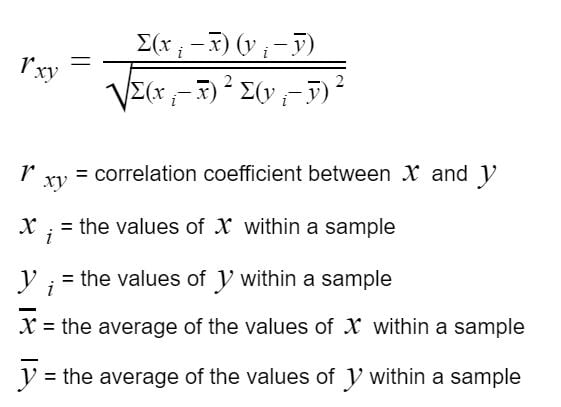
Iinear Correlation Coefficient

Direction:

• r > 0 → positive association.

• r < 0 → negative association

Form:

• r close to 0 = not linear.

Strength:

• The closer r is to ±1, the stronger the linear relationship.

• The closer r is to 0, the weaker the linear relationship.

*NOT RESISTANT

Correlation Coefficient and Critical Value

If the absolute value of the correlation coefficient is greater than the critical value, we say a linear relation exists between the two variables.

• Otherwise, there is no relation

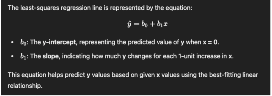
Least-Squares Regression

used to predict the value of the response variable (y) based on a given value of the explanatory variable (x)

• Creates linear equation (regression line)

• NOT FOR VALUES OUTSIDE RANGE OF DATA COLLECTED (extrapolation)

  

Extrapolation

the estimation of values beyond a known dataset's range

• can lead to answers that don’t make sense bc we cannot be certain of the behavior of data for which we have no observations

Residuals

prediction error for any given value of x.

• Formula: Residual = Observed y - Predicted y

• In a scatterplot, the residual is the vertical distance between a data point and the regression line (smaller distance the better)

R² (coefficient of determination)

Evaluates strength fit of a linear model

• calculated with square of correlation coefficient

• tells us what percent variability in response variable is explained in model

Limitations of Regression Models

• Approximation- average value of y given x, not exact

• Influence of Other Variables

• Random Variation- will be unexplained random variation in y

• Line of Means- regression line predicts mean value of y for all specific x

Probability Experiment

act or process of observation with uncertain results that can be repeated

• Probability of outcome- proportion of times that the outcome would occur in a long run of observations

• Probabilities are ALWAYS between 0 and 1

Independent Random Experiment

if the outcome of any one trial is not affected by the outcome of any other trial

• Ex. No matter how many times heads or tails have appeared before, the 11th flip is still a new event, and the probability of getting heads or tails remains 50%

Probability Model

Description of probability experiment, includes:

• list of all possible outcomes (sample space (S))

• probability for each outcome

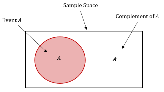
Sample Space

(denoted S) is the set of all possible outcomes

• Ex. Rolling a Die: S = {1, 2, 3, 4, 5, 6}

• Ex. Flipping a Coin: S = {H, T}

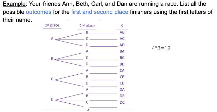
Tree Diagram

Sample space if experiment consist of more than one technique

• Ex. S = {HH, HT, TH, TT}

All Possible Outcomes Without Replacement

Multiply first and second amounts in tree graph

All Possible Outcomes With Replacement

Multiplication Rule for Counting: n^r

• repeating task with n outcomes r times

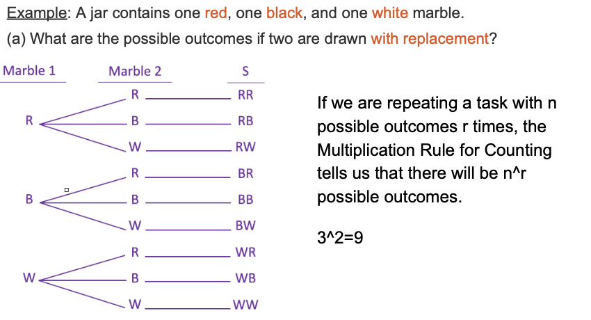
(3 marble types taken 2 times —> 3² = 9)

Event

any collection of outcomes from a probability experiment

• Denoted A or B

• impossible event- the probability of the event is 0

• certainty event- the probability of the event is 1

• unusual event- low probability of occurring

  • Typically, an event with a probability less than 0.05 (or 5%)

Simple Events

events w only one outcome denoted e

Equally Likely Outcomes

when each outcome has the same chance of occurring

Probability Range

Probability of event A (denoted as P(A)) must be between 0 and 1

• 0 < P(A) < 1

Sum of Probabilities

Sum of probabilities of all possible outcomes must equal 1

• If S = {e₁, e₂, e₃}, P(e₁) + P(e₂) + P(e₃) = 1

Complement

consists of all outcomes in the sample space that are not in event A.

• denote with A^c

• P(A^c) = 1 - P(A)

Mutually Exclusive Events

Disjointed- do not have any common outcomes

• P(A or(U) B) = P(A) + P(B)

Intersection Event

two events A and B consists of the outcomes in both A and B.

• ONLY THE OVERLAP (A and B at once)

• P(A ∩ B) = P(A) x P(B)

Union Event

two events A and B consists of outcomes that are in A or B.

• P(A or B) = A or B or Both

• P(A ∪ B) = P(A) + P(B) - P(A ∩ B)

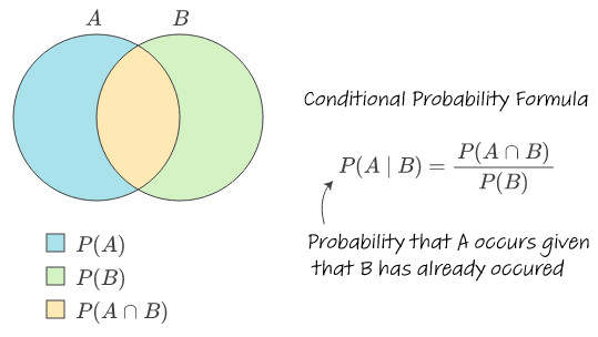
Conditional Probability

Of the cases in which B occurred, P(A|B) is the proportion in which A also occurred

• P(A and B) / P(B)

• Finding probability of event when you know what the outcome was for another event

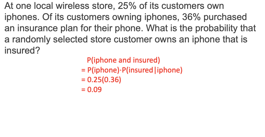
General Multiplication Rule

• P(A and B) = P(A|B) x P(B) or

• P(A and B) = P(B|A) x P(A)

3 Ways to Determine if A and B are independent events

1. Is P(A|B) = P(A)?

2. Is P(B|A) = P(B)?

3. Is P(A and B) = P(A)∙P(B)?

If any true, others true and they are independent